Lecture slides

Twelve Beamer decks live in Chapters/chapter_NN/, each folder self-contained: chapter_NN.tex, its images/, the compiled chapter_NN.pdf — and the companion lab for that chapter, so everything for one week sits together. The PDFs below are served with this documentation.

1027 slides in the main flow +139 in optional appendices 86 short + 41 extended exercises ~100 purpose-built figures

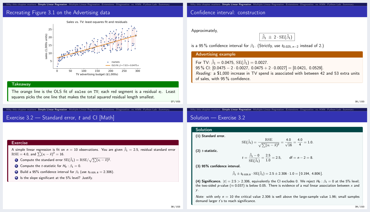
What a deck looks like: a figure computed from the course data with its takeaway, a worked example with real numbers, an in-deck exercise, and the worked solution that follows it two slides later.

The decks

Page counts are given as main flow and (appendix): every deck ends with an appendix of optional, more advanced material that the main thread never depends on — see what each appendix holds.

Ch.	Deck	What it covers	Exercises	Slides	PDF
0	Precourse (a) — Statistics refresher	Descriptive statistics, probability and Bayes, distributions, standard errors and confidence intervals, testing and power, simple regression, the Python toolkit	10 + 4	106 (+16)	Open
0b	Precourse (b) — Toolkit	Reading notation, logs and exponentials, odds and the logit, likelihood, computational cost, the Python patterns the labs use	6 + 2	51 (+9)	Open
1	Introduction	What statistical learning is, prediction vs. inference, the three motivating data sets, notation and the design matrix	3 + 1	71 (+6)	Open
2	Statistical Learning	Estimating f, parametric vs. nonparametric, the flexibility trade-off, training vs. test error, bias–variance, the Bayes classifier and KNN	8 + 4	107 (+8)	Open
3	Linear Regression	Least squares, standard errors and t/F inference, confidence vs. prediction intervals, dummies and interactions, the four diagnostics, KNN regression	12 + 6	144 (+11)	Open
4	Classification	Logistic regression and the odds scale, multiple predictors and confounding, the confusion matrix, ROC and AUC — the generative models (LDA, QDA, naive Bayes) now sit in the appendix	10 + 6	82 (+43)	Open
5	Resampling Methods	The validation set and why it wobbles, LOOCV, k-fold CV and the trade-off inside the estimate, CV pitfalls, the bootstrap	6 + 3	79 (+7)	Open
6	Model Selection & Regularization	Best subset and stepwise selection, Cₚ/AIC/BIC/adjusted R², ridge, the lasso and its sparsity, PCR, the p > n regime	7 + 3	81 (+11)	Open
7	Moving Beyond Linearity	Polynomials and step functions, regression splines and knots, natural splines, smoothing splines, LOESS, GAMs	6 + 3	85 (+7)	Open
8	Tree-Based Methods	Recursive binary splitting, pruning, classification trees and impurity, bagging and out-of-bag error, random forests, boosting	7 + 3	83 (+7)	Open
10	Deep Learning	Single-layer networks and activations, MLPs and parameter counts, convolutions and pooling, loss and SGD, regularisation and dropout	6 + 3	75 (+8)	Open
13	Multiple Testing	Why naive testing fails at scale, FWER, Bonferroni and Holm, the false discovery rate, Benjamini–Hochberg, p-hacking	5 + 3	63 (+6)	Open
Total			86 + 41	1027 (+139)

How a deck is built

Every deck follows the same rhythm, so students always know where they are.

1. Front matter — course-at-a-glance, chapter contents, and a “Notation in this chapter” symbol table.

2. Teaching flow — motivation → intuition → formal definition → worked example → interpretation, with colour-coded callout boxes:

   Box	Meaning
   🟩 green	Takeaway — the sentence to remember
   🟦 blue	How to read this — a formula explained symbol by symbol
   🟧 orange	Worked example with concrete numbers
   🟥 red	Common pitfall
   🟪 purple	Short exercise (~5 min) · 🟩 teal = its solution
   🟣 violet	Extended exercise (~15 min)
   🩵 cyan	“Companion notebook” — switch to the Jupyter lab now

3. Exercises — roughly one short exercise every 20 minutes and one extended exercise every 45 minutes, each tagged [Concept] / [Math] / [Python] (short) or [Math] / [Python] / [Integrative] (extended), so you can pick the right mix for your room. Every prompt is followed by its worked solution; long ones run across a clean (1/2) / (2/2) pair.

4. Closing summary — chapter-in-one-slide, key formulas at a glance, vocabulary, decision rules and common pitfalls.

5. Appendix — the optional, more advanced material, opened by a slide that says what is in it and why each item is optional.

Two things hold throughout:

• ~100 purpose-built visuals — 65 matplotlib plots generated from the bundled datasets plus 39 native TikZ concept diagrams. Among them: the bias–variance trade-off, the logistic S-curve, ROC and a confusion-matrix schematic, k-fold and bootstrap diagrams, ridge & lasso coefficient paths with the \(\ell_1\)-vs-\(\ell_2\) constraint geometry, spline/GAM fits, a decision tree beside its feature-space partition, a neural-network architecture, a convolution diagram, and the Benjamini–Hochberg staircase.

• Verified numbers — Python listings are commented and runnable against the bundled datasets, and every numeric answer was reproduced against the real data.

What each appendix holds

The appendix sits outside the timed plan: the runsheets stop where it begins, and the slide index marks it optional rather than budgeting minutes for it. Every exercise in an appendix keeps its full solution, so it works as homework.

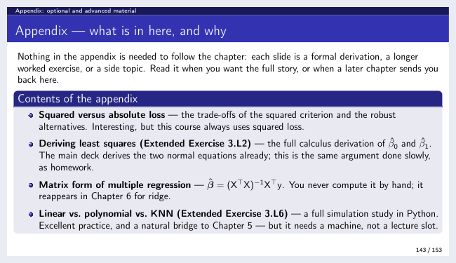
Every appendix opens with this slide: what is in it, and why each item is optional.

Ch.	In its appendix	Pages
0	χ²/t/F and LLN vs. CLT · the ANOVA decomposition · linear algebra (with Exercise 0.8) · calculus and gradient descent (with Extended Exercise 0.3)	16
0b	least squares as maximum likelihood (with Extended Exercise 0b.1) · counting and the 2ᵖ cost (with Exercise 0b.5)	9
1	the design matrix entry by entry · the two dataset lookup tables	6
2	Extended Exercise 2.1 (bias–variance from first principles) · Extended Exercise 2.3 (the Bayes boundary for two Gaussians)	8
3	squared vs. absolute loss · Extended Exercise 3.L2 (deriving least squares) · the matrix form of multiple regression · Extended Exercise 3.L6 (linear vs. polynomial vs. KNN)	11
4	how logistic regression is actually fitted (deviance, IRLS) · the multinomial softmax · the generative models in full — Bayes refresher, LDA, QDA, naive Bayes, with Exercises 4.5–4.7 · Extended Exercise 4.2 (LDA from Bayes’ theorem) · Extended Exercise 4.3 (naive Bayes by hand) · comparing the classifiers, with Extended Exercise 4.4 · GLMs and Poisson regression	43
5	Exercise 5.2 and Extended Exercise 5.1 — the LOOCV leverage-shortcut drills	7
6	the constraint geometry redrawn · Exercise 6.1 (counting models) · Extended Exercise 6.2 (orthonormal design, soft thresholding) · partial least squares with Exercise 6.6	11
7	the truncated-power basis and the constraint count · Extended Exercise 7.1 (regression splines by hand)	7
8	the partition picture redrawn · Extended Exercise 8.2 (impurity measures and pruning) · BART	7
10	Extended Exercise 10.2 (CNN architecture arithmetic) · transformers · backpropagation · double descent	8
13	the four outcomes drawn · resampling-based inference · post-selection inference	6

The two precourse decks

Both are taught, in the single precourse session that opens the semester, and both exist because the ten chapter decks assume their content silently. One session cannot cover 157 slides, so it draws a selection from the two and the decks remain the full reference — see the course at a glance and For students.

Chapter 0 — the statistics refresher

For students who need the undergraduate material back, and for anyone teaching a cohort with mixed backgrounds. It covers:

• data and variable types; centre, spread and shape; boxplots and \(z\)-scores;

• covariance, correlation and what correlation cannot see; confounding;

• probability rules, conditional probability and Bayes’ theorem (with the base-rate trap that motivates Chapter 4’s ROC curves);

• the Bernoulli, binomial, Poisson and normal distributions, and the central limit theorem;

• standard errors, confidence intervals, hypothesis tests and the standard misreadings of both;

• simple linear regression end to end: least squares, residuals, \(R^2\);

• the numpy / pandas / matplotlib / statsmodels / scikit-learn toolkit of the labs.

The linear algebra and the calculus/gradient-descent strands sit in its appendix, for the cohorts that need them. It opens with a twelve-question self-check so students can decide whether they need the session at all, and closes with a table mapping every topic to the chapter that uses it. Eighteen figures — the boxplot anatomy, a gallery of shapes, Anscombe’s quartet, Simpson’s paradox, the CLT, confidence-interval coverage, \(p\)-values as areas, power, leverage, and gradient descent on a real loss surface — are computed from the course data by Chapters/chapter_00/make_figures.py, and every one is rebuilt in code in the companion notebook.

Chapter 0b — the toolkit

Covering what the ten lecture decks use but never explain. Its scope was not guessed — it comes from counting usage across the decks:

Topic	Where it bites	Uses
log and exp	Ch. 4 (113), Ch. 10 (31), Ch. 6 (16)	176
odds and the logit	Ch. 4 (92), Ch. 10 (12)	108
likelihood and ∏	Ch. 4 (35), Ch. 2–3	37
∑, arg max, indicators, sets	every chapter from Ch. 2	180
counting and the 2ᵖ cost	Ch. 6 (subset selection)	13

It adds a sixth strand the labs depend on and the decks never teach: the Python patterns themselves — writing a function, looping over candidate settings, seeding randomness, the fit/predict contract, and the discipline of scoring on data the model has not seen. Eight figures, six short and two extended exercises, and a companion notebook. The maximum-likelihood derivation and the counting strand live in its appendix.

Rebuilding a deck

Requires a TeX Live distribution with beamer, tcolorbox, tikz, listings and booktabs:

cd Chapters/chapter_08
pdflatex chapter_08.tex
pdflatex chapter_08.tex   # second pass for the navigation bar

From the repository root, make rebuilds every deck whose source changed and refreshes the slide index, and make check reports page counts and any slide that overruns its frame. Python snippets inside the slides read data from ../../ALL CSV FILES - 2nd Edition/ or via the ISLP package.

Figures from the book

Decks that reproduce a textbook figure attribute it to its source. The copyrighted textbook PDF and figure banks (Source_Material/) are not included in the repository.

Where to go next

• Lab notebooks — the companion notebook for each deck.

• Teaching it — runsheets, the slide index, and how the appendix fits a session.

• The course at a glance — which deck goes in which week.