This notebook runs on Colab as-is. The badge link above and the GITHUB_RAW line in the setup cell already point to this repository, so everything installs and loads automatically.

Chapter 2 — Statistical Learning

Lab: NumPy, pandas, plotting, KNN

Course: Quantitative Research Methods
Instructor: Prof. Dr. Christoph Weisser, HSBI
Source: James, Witten, Hastie, Tibshirani & Taylor (2023), An Introduction to Statistical Learning, with Applications in Python, Springer. Companion code at statlearning.com.

Goal of this lab. Get fluent with NumPy, pandas, and matplotlib; reproduce the bias–variance and KNN figures from the chapter; fit a KNN classifier with cross-validated \(K\).

Setup

Run this cell once. The ISLP package can be installed with pip install ISLP. As an alternative, the same data sets are available as CSVs in the workspace’s ALL CSV FILES - 2nd Edition folder.

Google Colab: this notebook also runs on Colab out of the box — the setup cell below installs any missing packages and downloads the data automatically.

# --- Setup: runs locally AND on Google Colab --------------------------------
# Silence only the spurious 'encountered in matmul' RuntimeWarnings that the macOS
# Accelerate BLAS emits; real warnings (deprecations, model caveats) stay visible.
import warnings
warnings.filterwarnings('ignore', message='.*encountered in matmul', category=RuntimeWarning)
import importlib.util, os, subprocess, sys

IN_COLAB = 'google.colab' in sys.modules

def _ensure(pkg, import_name=None):
    """pip-install pkg (quietly) if its import is missing."""
    if importlib.util.find_spec(import_name or pkg) is None:
        subprocess.run([sys.executable, '-m', 'pip', 'install', '-q', pkg], check=False)

if IN_COLAB:  # Colab ships numpy/pandas/sklearn/statsmodels; add course extras
    for _pkg, _imp in [('ISLP', 'ISLP')]:
        _ensure(_pkg, _imp)

import numpy as np
import pandas as pd
import matplotlib.pyplot as plt

rng = np.random.default_rng(2024)
plt.rcParams['figure.dpi'] = 110

try:
    from ISLP import load_data
    HAVE_ISLP = True
except ImportError:
    HAVE_ISLP = False
    print('ISLP not installed; using CSV / URL fallbacks.')

# Local CSV location (repo layout first, then legacy paths, then a data/ cache).
_CANDIDATES = ['../ALL CSV FILES - 2nd Edition',
               'ALL CSV FILES - 2nd Edition',
               '../../ALL CSV FILES - 2nd Edition', 'data']
CSV = next((p for p in _CANDIDATES if os.path.isdir(p)), 'data')

# GITHUB_RAW lets a fresh Colab runtime fetch any
# CSV that is neither in ISLP nor already local (spaces in the folder -> %20).
GITHUB_RAW = ('https://raw.githubusercontent.com/ChrisW09/Quantitative-Research-Methods/main/'
              'ALL%20CSV%20FILES%20-%202nd%20Edition')

# The four datasets NOT in the ISLP package -> load from the book's official
# site so the notebook works on a fresh Colab even before the repo is published.
KNOWN_URLS = {
    'Advertising': 'https://www.statlearning.com/s/Advertising.csv',
    'Heart':       'https://www.statlearning.com/s/Heart.csv',
    'Income1':     'https://www.statlearning.com/s/Income1.csv',
    'Income2':     'https://www.statlearning.com/s/Income2.csv',
}

def load(name, **read_csv_kwargs):
    """Load a course dataset. Order: ISLP package -> R datasets -> local CSV
    -> official book URL -> your GitHub repo. Works locally and on Colab."""
    if HAVE_ISLP:
        try:
            return load_data(name)
        except Exception:
            pass
    if name == 'USArrests':                       # classic R dataset, not in ISLP
        try:
            import statsmodels.api as sm
            return sm.datasets.get_rdataset('USArrests', 'datasets').data
        except Exception:
            pass
    path = f'{CSV}/{name}.csv'
    if os.path.exists(path):                      # running from the repo (local)
        return pd.read_csv(path, **read_csv_kwargs)
    remotes = ([KNOWN_URLS[name]] if name in KNOWN_URLS else []) + [f'{GITHUB_RAW}/{name}.csv']
    for url in remotes:                           # fresh Colab: stream over https
        try:
            return pd.read_csv(url, **read_csv_kwargs)
        except Exception:
            continue
    raise FileNotFoundError(
        f"Could not load {name!r}. Put the CSV in '{CSV}/' or check your connection for the GITHUB_RAW fallback.")

1. NumPy refresher

x = np.array([3, 4, 5])
y = np.array([4, 9, 7])
x.sum(), x.mean(), x.std(ddof=1)

(np.int64(12), np.float64(4.0), np.float64(1.0))

A = np.array([[1, 2], [3, 4]])
A.shape, A.T, np.linalg.inv(A), A @ A

((2, 2),
 array([[1, 3],
        [2, 4]]),
 array([[-2. ,  1. ],
        [ 1.5, -0.5]]),
 array([[ 7, 10],
        [15, 22]]))

z = rng.standard_normal(size=(100, 2))
z.mean(axis=0), z.std(axis=0, ddof=1)

(array([-0.1046211 ,  0.03985462]), array([1.00897462, 0.97285773]))

2. pandas

Auto = load('Auto', na_values='?').dropna()
Auto = Auto.reset_index(drop=True)
print(Auto.shape); Auto.head()

(392, 8)

	mpg	cylinders	displacement	horsepower	weight	acceleration	year	origin
0	18.0	8	307.0	130	3504	12.0	70	1
1	15.0	8	350.0	165	3693	11.5	70	1
2	18.0	8	318.0	150	3436	11.0	70	1
3	16.0	8	304.0	150	3433	12.0	70	1
4	17.0	8	302.0	140	3449	10.5	70	1

Auto.describe()

	mpg	cylinders	displacement	horsepower	weight	acceleration	year	origin
count	392.000000	392.000000	392.000000	392.000000	392.000000	392.000000	392.000000	392.000000
mean	23.445918	5.471939	194.411990	104.469388	2977.584184	15.541327	75.979592	1.576531
std	7.805007	1.705783	104.644004	38.491160	849.402560	2.758864	3.683737	0.805518
min	9.000000	3.000000	68.000000	46.000000	1613.000000	8.000000	70.000000	1.000000
25%	17.000000	4.000000	105.000000	75.000000	2225.250000	13.775000	73.000000	1.000000
50%	22.750000	4.000000	151.000000	93.500000	2803.500000	15.500000	76.000000	1.000000
75%	29.000000	8.000000	275.750000	126.000000	3614.750000	17.025000	79.000000	2.000000
max	46.600000	8.000000	455.000000	230.000000	5140.000000	24.800000	82.000000	3.000000

Auto.groupby('origin')['mpg'].agg(['mean', 'std', 'count'])

	mean	std	count
origin
1	20.033469	6.440384	245
2	27.602941	6.580182	68
3	30.450633	6.090048	79

3. Plots

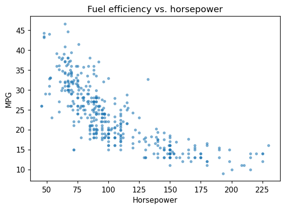
fig, ax = plt.subplots(figsize=(6, 4))
ax.scatter(Auto['horsepower'], Auto['mpg'], s=8, alpha=0.5)
ax.set(xlabel='Horsepower', ylabel='MPG',
       title='Fuel efficiency vs. horsepower')
plt.show()

import seaborn as sns
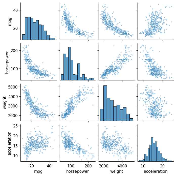
sns.pairplot(Auto[['mpg', 'horsepower', 'weight', 'acceleration']],
             height=1.6, plot_kws=dict(s=8, alpha=0.4))
plt.show()

4. Reproducing Figure 2.9 — bias–variance

Simulate, fit a linear regression and two splines, plot training and test MSE.

from sklearn.preprocessing import SplineTransformer
from sklearn.linear_model import LinearRegression
from sklearn.pipeline import make_pipeline
from sklearn.metrics import mean_squared_error

def make_data(n=80, seed=0):
    rng = np.random.default_rng(seed)
    x = np.sort(rng.uniform(-3, 3, size=n))
    f = np.sin(x) + 0.3*x
    y = f + rng.normal(scale=0.4, size=n)
    return x.reshape(-1, 1), y, f

X_tr, y_tr, f_tr = make_data(80, seed=0)
X_te, y_te, f_te = make_data(400, seed=1)

models = {
    'linear': LinearRegression(),
    'spline df=4': make_pipeline(SplineTransformer(degree=3, n_knots=4),
                                  LinearRegression()),
    'spline df=10': make_pipeline(SplineTransformer(degree=3, n_knots=10),
                                   LinearRegression()),
}

fig, axes = plt.subplots(1, 2, figsize=(11, 4))
axes[0].scatter(X_tr, y_tr, s=10, color='black')
for name, mdl in models.items():
    mdl.fit(X_tr, y_tr)
    grid = np.linspace(-3, 3, 200).reshape(-1, 1)
    axes[0].plot(grid, mdl.predict(grid), label=name)
axes[0].legend(); axes[0].set_title('Fits')

df_grid = list(range(2, 25))
tr_mse, te_mse = [], []
for k in df_grid:
    m = make_pipeline(SplineTransformer(degree=3, n_knots=max(2, k - 2)),
                      LinearRegression()).fit(X_tr, y_tr)
    tr_mse.append(mean_squared_error(y_tr, m.predict(X_tr)))
    te_mse.append(mean_squared_error(y_te, m.predict(X_te)))
axes[1].plot(df_grid, tr_mse, label='train MSE')
axes[1].plot(df_grid, te_mse, label='test MSE')
axes[1].axhline(0.16, ls='--', color='grey', label='Var(eps)')
axes[1].set(xlabel='effective df', ylabel='MSE'); axes[1].legend()
plt.tight_layout(); plt.show()

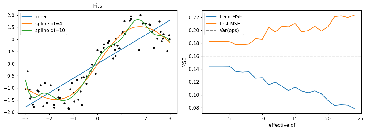
Test MSE has the predicted U-shape; training MSE never increases.

5. KNN classification

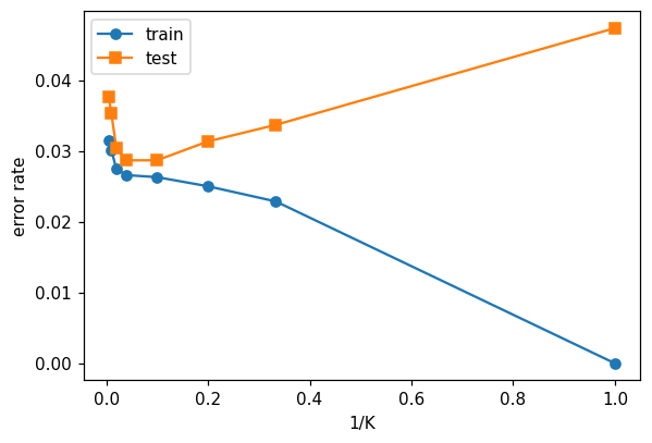
Reproduce the classification U-curve (Figure 2.17) on the Default data.

from sklearn.neighbors import KNeighborsClassifier
from sklearn.model_selection import train_test_split
from sklearn.preprocessing import StandardScaler

Default = load('Default')
y = (Default['default'] == 'Yes').astype(int).values
X = Default[['balance', 'income']].values
Xtr, Xte, ytr, yte = train_test_split(X, y, test_size=0.3,
                                       random_state=0)
scaler = StandardScaler().fit(Xtr)
Xtr_s = scaler.transform(Xtr); Xte_s = scaler.transform(Xte)

ks = np.array([1, 3, 5, 10, 25, 50, 100, 200])
tr_err, te_err = [], []
for k in ks:
    knn = KNeighborsClassifier(n_neighbors=int(k)).fit(Xtr_s, ytr)
    tr_err.append(1 - knn.score(Xtr_s, ytr))
    te_err.append(1 - knn.score(Xte_s, yte))

fig, ax = plt.subplots(figsize=(6, 4))
ax.plot(1/ks, tr_err, marker='o', label='train')
ax.plot(1/ks, te_err, marker='s', label='test')
ax.set(xlabel='1/K', ylabel='error rate'); ax.legend()
plt.show()

Lecture exercises — worked Python solutions

The chapter 2 slide deck tags two exercises as [Python]: Exercise 2.8 — Scatter and flexibility on Auto and Extended Exercise 2.2 — KNN simulation study. Both are mirrored here as fully worked, runnable solutions. The code uses the load() helper from the setup cell (never hard-coded paths), and the numeric results quoted on the slides are noted as trailing comments.

Exercise 2.8 — Scatter and flexibility on Auto (slide: Exercise 2.8 [Python])

Load the Auto data, make a scatter plot of mpg (y-axis) against horsepower (x-axis), and comment on what level of flexibility a good model of this relationship needs. Note that horsepower contains a few "?" missing entries you must handle.

# Exercise 2.8 — worked solution ------------------------------------------------
# Load via the course helper (ISLP package if installed, else the bundled CSVs).
Auto28 = load('Auto')

# In the raw CSV the '?' entries make pandas read horsepower as strings
# (dtype object). Handle them exactly as on the slide: drop those rows, then
# convert to float. (The ISLP copy is already numeric, so this branch is a no-op.)
if Auto28['horsepower'].dtype == object:
    Auto28 = Auto28[Auto28['horsepower'] != '?'].copy()      # drops 5 missing rows
    Auto28['horsepower'] = Auto28['horsepower'].astype(float)

fig, ax = plt.subplots(figsize=(6, 4))
ax.scatter(Auto28['horsepower'], Auto28['mpg'], s=10)
ax.set_xlabel('horsepower'); ax.set_ylabel('mpg')
ax.set_title('Auto: mpg vs. horsepower')
plt.show()

print('n =', Auto28.shape[0])                                # expected: 392
print('corr =', round(Auto28['horsepower'].corr(Auto28['mpg']), 2)) # expected: -0.78

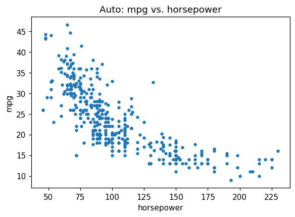
n = 392
corr = -0.78

Interpretation (as on the slide). After dropping the 5 missing rows, \(n = 392\). The cloud is clearly nonlinear: mpg falls steeply as horsepower rises and then flattens (a convex, decreasing curve; correlation \(\approx -0.78\)). A straight line would underfit this curvature (high bias); a moderately flexible fit — a quadratic/polynomial or a spline — captures it well; an extremely flexible fit that wiggles through every point would overfit (high variance).

Extended Exercise 2.2 — KNN simulation study (slide: Extended Exercise 2.2 [Python])

Build a controlled experiment that exposes the bias–variance trade-off in KNN.

1. Simulate a 2-class 2-D problem: class 0 from \(\mathcal{N}((0,0), I)\) and class 1 from \(\mathcal{N}((2,2), I)\). Draw \(n_{\text{train}} = 200\) and a large \(n_{\text{test}} = 2000\) (half per class).

2. For \(K = 1, 2, \ldots, 50\) fit a \(K\)-NN classifier and record the training and test error rates.

3. Plot both errors against \(1/K\) (flexibility) and identify the \(K\) that minimises test error.

4. Explain each curve via bias and variance, and compare the best test error to the Bayes rate \(\Phi(-\sqrt{2}) \approx 0.079\) (means \(2\sqrt{2}\) apart, unit variance).

# Extended Exercise 2.2 — worked solution (parts 1-2) ----------------------------
from sklearn.neighbors import KNeighborsClassifier

rng22 = np.random.default_rng(1)      # the slide's seed -> reproduces its numbers

def sample(n):
    """Draw n points, half per class: class 0 ~ N((0,0), I), class 1 ~ N((2,2), I)."""
    n0 = n // 2
    X = np.vstack([rng22.normal([0, 0], 1, (n0, 2)),        # class 0, centre (0,0)
                   rng22.normal([2, 2], 1, (n - n0, 2))])   # class 1, centre (2,2)
    y = np.r_[np.zeros(n0), np.ones(n - n0)]
    return X, y

Xtr, ytr = sample(200)     # training set (drawn FIRST -- the draw order matters
Xte, yte = sample(2000)    # for reproducing the seeded numbers), then the test set

Ks = range(1, 51)
tr_err, te_err = [], []
for K in Ks:                                    # (2) fit KNN for K = 1..50
    knn = KNeighborsClassifier(n_neighbors=K).fit(Xtr, ytr)
    tr_err.append(1 - knn.score(Xtr, ytr))      # error rate = 1 - accuracy
    te_err.append(1 - knn.score(Xte, yte))

best_K = int(np.argmin(te_err)) + 1
print('best K =', best_K, '  min test err =', round(min(te_err), 3))
# expected (this seed): best K = 14   min test err = 0.076
print('train err at K=1 :', round(tr_err[0], 3))     # expected: 0.0  (memorises)
print('train err at K=50:', round(tr_err[-1], 3))    # expected: 0.035
print('test  err at K=1 :', round(te_err[0], 3))     # expected: 0.093

best K = 14   min test err = 0.076
train err at K=1 : 0.0
train err at K=50: 0.035
test  err at K=1 : 0.093

# Extended Exercise 2.2 — worked solution (parts 3-4) ----------------------------
# Bayes rate for two unit-variance Gaussians whose means are 2*sqrt(2) apart:
# Phi(-sqrt(2)) -- the irreducible floor for ANY classifier on this problem.
from scipy.stats import norm
bayes = norm.cdf(-np.sqrt(2))
print('Bayes error rate =', round(bayes, 3))          # expected: 0.079

inv_K = [1 / K for K in Ks]                           # x-axis: flexibility = 1/K
fig, ax = plt.subplots(figsize=(6.5, 4))
ax.plot(inv_K, tr_err, marker='.', label='training error')
ax.plot(inv_K, te_err, marker='.', label='test error')
ax.axhline(bayes, ls='--', color='grey', label=f'Bayes rate ~ {bayes:.3f}')
ax.axvline(1 / best_K, ls=':', color='red', label=f'best K = {best_K}')
ax.set_xlabel('1/K  (flexibility)'); ax.set_ylabel('error rate')
ax.legend(); plt.show()
# Expected picture: training error falls to 0 as 1/K -> 1 (K = 1 memorises);
# test error is U-shaped with its minimum near K = 10-20, essentially at the
# Bayes floor.

Bayes error rate = 0.079

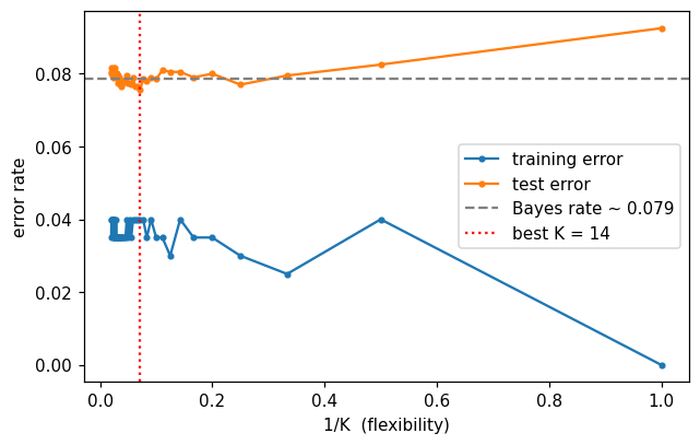
Reading the curves (as on the slide). With this seed the best \(K \approx 14\) with test error \(\approx 0.076\) — essentially the Bayes floor \(\approx 0.079\).

• Training error climbs from \(0\) at \(K=1\) (each point is its own nearest neighbour) to \(\approx 0.035\) at \(K=50\); it does not track test error.

• Test error is U-shaped in \(1/K\): worst at \(K=1\) (\(\approx 0.093\), high variance), dips near \(K \approx 10\)–\(20\), then drifts up for very large \(K\) (rising bias).

Small \(K\) = flexible = low bias, high variance; large \(K\) = rigid = high bias, low variance. Cross-validation would pick a \(K\) in the flat basin at the bottom.

6. Exercises

1. Repeat the bias–variance simulation with a noisier truth (scale=0.8). Where does the U-curve minimum move?

2. Replace sin(x) + 0.3*x with a near-linear truth 0.5*x + 1. Verify that the linear model now wins.

3. Standardise Default with RobustScaler instead of StandardScaler. Does \(K^*\) change?

4. Add student (binary) as a third predictor in the Default KNN. Does test error improve?