
This notebook runs on Colab as-is. The badge link above and the GITHUB_RAW line in the setup cell already point to this repository, so everything installs and loads automatically.
Chapter 4 — Classification
Lab: logistic regression, LDA, QDA, naive Bayes, ROC, Poisson
Course: Quantitative Research Methods
Instructor: Prof. Dr. Christoph Weisser, HSBI
Source: James, Witten, Hastie, Tibshirani & Taylor (2023), An Introduction to Statistical Learning, with Applications in Python, Springer. Companion code at statlearning.com.
Goal of this lab. Fit five different classifiers on the Default and Smarket data, compare them via confusion matrices and ROC curves, and run a Poisson regression on Bikeshare.
Setup
Run this cell once. The ISLP package can be installed with pip install ISLP. As an alternative, the same data sets are available as CSVs in the workspace’s ALL CSV FILES - 2nd Edition folder.
Google Colab: this notebook also runs on Colab out of the box — the setup cell below installs any missing packages and downloads the data automatically.
# --- Setup: runs locally AND on Google Colab --------------------------------
# Silence only the spurious 'encountered in matmul' RuntimeWarnings that the macOS
# Accelerate BLAS emits; real warnings (deprecations, model caveats) stay visible.
import warnings
warnings.filterwarnings('ignore', message='.*encountered in matmul', category=RuntimeWarning)
import importlib.util, os, subprocess, sys

IN_COLAB = 'google.colab' in sys.modules

def _ensure(pkg, import_name=None):
    """pip-install pkg (quietly) if its import is missing."""
    if importlib.util.find_spec(import_name or pkg) is None:
        subprocess.run([sys.executable, '-m', 'pip', 'install', '-q', pkg], check=False)

if IN_COLAB:  # Colab ships numpy/pandas/sklearn/statsmodels; add course extras
    for _pkg, _imp in [('ISLP', 'ISLP')]:
        _ensure(_pkg, _imp)

import numpy as np
import pandas as pd
import matplotlib.pyplot as plt

rng = np.random.default_rng(2024)
plt.rcParams['figure.dpi'] = 110

try:
    from ISLP import load_data
    HAVE_ISLP = True
except ImportError:
    HAVE_ISLP = False
    print('ISLP not installed; using CSV / URL fallbacks.')

# Local CSV location (repo layout first, then legacy paths, then a data/ cache).
_CANDIDATES = ['../ALL CSV FILES - 2nd Edition',
               'ALL CSV FILES - 2nd Edition',
               '../../ALL CSV FILES - 2nd Edition', 'data']
CSV = next((p for p in _CANDIDATES if os.path.isdir(p)), 'data')

# GITHUB_RAW lets a fresh Colab runtime fetch any
# CSV that is neither in ISLP nor already local (spaces in the folder -> %20).
GITHUB_RAW = ('https://raw.githubusercontent.com/ChrisW09/Quantitative-Research-Methods/main/'
              'ALL%20CSV%20FILES%20-%202nd%20Edition')

# The four datasets NOT in the ISLP package -> load from the book's official
# site so the notebook works on a fresh Colab even before the repo is published.
KNOWN_URLS = {
    'Advertising': 'https://www.statlearning.com/s/Advertising.csv',
    'Heart':       'https://www.statlearning.com/s/Heart.csv',
    'Income1':     'https://www.statlearning.com/s/Income1.csv',
    'Income2':     'https://www.statlearning.com/s/Income2.csv',
}

def load(name, **read_csv_kwargs):
    """Load a course dataset. Order: ISLP package -> R datasets -> local CSV
    -> official book URL -> your GitHub repo. Works locally and on Colab."""
    if HAVE_ISLP:
        try:
            return load_data(name)
        except Exception:
            pass
    if name == 'USArrests':                       # classic R dataset, not in ISLP
        try:
            import statsmodels.api as sm
            return sm.datasets.get_rdataset('USArrests', 'datasets').data
        except Exception:
            pass
    path = f'{CSV}/{name}.csv'
    if os.path.exists(path):                      # running from the repo (local)
        return pd.read_csv(path, **read_csv_kwargs)
    remotes = ([KNOWN_URLS[name]] if name in KNOWN_URLS else []) + [f'{GITHUB_RAW}/{name}.csv']
    for url in remotes:                           # fresh Colab: stream over https
        try:
            return pd.read_csv(url, **read_csv_kwargs)
        except Exception:
            continue
    raise FileNotFoundError(
        f"Could not load {name!r}. Put the CSV in '{CSV}/' or check your connection for the GITHUB_RAW fallback.")
1. Logistic regression
import statsmodels.api as sm
Default = load('Default')
y = (Default['default'] == 'Yes').astype(int)
Default['student_d'] = (Default['student'] == 'Yes').astype(int)
X = sm.add_constant(Default[['balance', 'income', 'student_d']])
res = sm.GLM(y, X, family=sm.families.Binomial()).fit()
print(res.summary())
                 Generalized Linear Model Regression Results
==============================================================================
Dep. Variable:                default   No. Observations:                10000
Model:                            GLM   Df Residuals:                     9996
Model Family:                Binomial   Df Model:                            3
Link Function:                  Logit   Scale:                          1.0000
Method:                          IRLS   Log-Likelihood:                -785.77
Date:                Sun, 19 Jul 2026   Deviance:                       1571.5
Time:                        14:31:49   Pearson chi2:                 7.00e+03
No. Iterations:                     9   Pseudo R-squ. (CS):             0.1262
Covariance Type:            nonrobust
==============================================================================
                 coef    std err          z      P>|z|      [0.025      0.975]
------------------------------------------------------------------------------
const        -10.8690      0.492    -22.079      0.000     -11.834      -9.904
balance        0.0057      0.000     24.737      0.000       0.005       0.006
income      3.033e-06    8.2e-06      0.370      0.712    -1.3e-05    1.91e-05
student_d     -0.6468      0.236     -2.738      0.006      -1.110      -0.184
==============================================================================
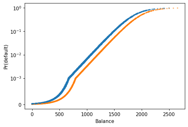
Note that student_d flips sign once balance is held constant — the textbook’s student paradox.
Predicted probabilities
p = res.predict(X)
fig, ax = plt.subplots(figsize=(6, 4))
ax.scatter(Default['balance'], p, s=4, alpha=0.4,
            c=Default['student_d'].map({0: 'C0', 1: 'C1'}))
ax.set(xlabel='Balance', ylabel='Pr(default)')
ax.set_yscale('symlog', linthresh=1e-3); plt.show()
2. LDA, QDA, naive Bayes, KNN — head-to-head
from sklearn.model_selection import train_test_split
from sklearn.preprocessing import StandardScaler
from sklearn.linear_model import LogisticRegression
from sklearn.discriminant_analysis import (
    LinearDiscriminantAnalysis as LDA,
    QuadraticDiscriminantAnalysis as QDA)
from sklearn.naive_bayes import GaussianNB
from sklearn.neighbors import KNeighborsClassifier
from sklearn.metrics import classification_report, roc_auc_score

X = Default[['balance', 'income', 'student_d']].values
y = (Default['default'] == 'Yes').astype(int).values
Xtr, Xte, ytr, yte = train_test_split(X, y, test_size=0.3, random_state=0)
scaler = StandardScaler().fit(Xtr)
Xtr_s, Xte_s = scaler.transform(Xtr), scaler.transform(Xte)

models = {
    'logit': LogisticRegression(max_iter=2000),
    'LDA':   LDA(),
    'QDA':   QDA(),
    'NB':    GaussianNB(),
    'KNN5':  KNeighborsClassifier(n_neighbors=5),
}

for name, mdl in models.items():
    mdl.fit(Xtr_s, ytr)
    proba = mdl.predict_proba(Xte_s)[:, 1]
    print(f'{name:6s}  AUC = {roc_auc_score(yte, proba):.3f}')
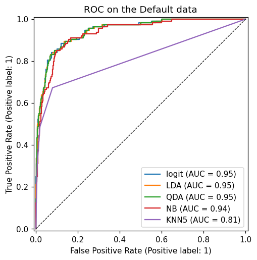
logit   AUC = 0.946
LDA     AUC = 0.946
QDA     AUC = 0.946
NB      AUC = 0.935
KNN5    AUC = 0.811
ROC curves
from sklearn.metrics import RocCurveDisplay
fig, ax = plt.subplots(figsize=(5, 5))
for name, mdl in models.items():
    RocCurveDisplay.from_estimator(mdl, Xte_s, yte, ax=ax, name=name)
ax.plot([0, 1], [0, 1], 'k--', lw=0.8)
ax.set_title('ROC on the Default data'); plt.show()
Lecture exercises — worked Python solutions
Runnable, verified solutions to the three [Python]-tagged exercises in the Chapter 4 lecture deck. Each cell uses the load() helper from the Setup cell above (no hard-coded paths), and the reported numbers match the slide solutions.
Extended Exercise 4.5 — Default: logistic regression, confusion matrix, ROC/AUC
Using the Default data: (1) fit a logistic regression of default on balance, income and a 0/1 student indicator; (2) build the confusion matrix at thresholds 0.5 and 0.2; (3) at each threshold report accuracy, sensitivity, specificity and precision; (4) plot the ROC curve and report the AUC.
# Extended Exercise 4.5 — Default: logistic regression, confusion matrix, ROC/AUC
from sklearn.linear_model import LogisticRegression
from sklearn.metrics import confusion_matrix, roc_auc_score, RocCurveDisplay

Default = load('Default')                                # setup-cell helper (ISLP -> CSV)
y = (Default['default'] == 'Yes').astype(int)            # encode response as 0/1
X = Default.assign(stud=(Default['student'] == 'Yes').astype(int)
                   )[['balance', 'income', 'stud']].values   # predictors incl. student dummy

clf   = LogisticRegression(max_iter=10000).fit(X, y)     # fit by (penalised) maximum likelihood
proba = clf.predict_proba(X)[:, 1]                        # predicted P(default = Yes) per customer

# metrics at two decision thresholds (sklearn orders cells as TN, FP, FN, TP)
print(f"{'t':>4} {'TN':>5} {'FP':>4} {'FN':>4} {'TP':>4}  {'acc':>5} {'sens':>5} {'spec':>5} {'prec':>5}")
for t in (0.5, 0.2):
    tn, fp, fn, tp = confusion_matrix(y, proba > t).ravel()
    sens, spec = tp/(tp+fn), tn/(tn+fp)                  # sensitivity, specificity
    prec, acc  = tp/(tp+fp), (tp+tn)/len(y)              # precision, accuracy
    print(f"{t:>4} {tn:>5} {fp:>4} {fn:>4} {tp:>4}  "
          f"{acc:>5.3f} {sens:>5.3f} {spec:>5.3f} {prec:>5.3f}")

print('AUC =', round(roc_auc_score(y, proba), 3))        # threshold-free ranking quality
RocCurveDisplay.from_predictions(y, proba)               # draw the ROC curve
plt.title('Default — logistic regression ROC'); plt.show()

# Expected output (matches slide Extended Exercise 4.5):
#     t    TN   FP   FN   TP    acc  sens  spec  prec
#   0.5  9627   40  228  105  0.973 0.315 0.996 0.724
#   0.2  9390  277  130  203  0.959 0.610 0.971 0.423
#   AUC = 0.95
   t    TN   FP   FN   TP    acc  sens  spec  prec
 0.5  9627   40  228  105  0.973 0.315 0.996 0.724
 0.2  9390  277  130  203  0.959 0.610 0.971 0.423
AUC = 0.95
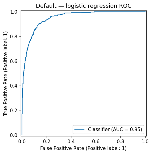
At threshold 0.5 the model is accurate (97.3%) but has low sensitivity (0.315) — it misses about two-thirds of true defaulters, the always-predict-No trap on imbalanced data. Lowering the threshold to 0.2 nearly doubles sensitivity (0.610) at the cost of specificity (0.996 → 0.971) and precision (0.724 → 0.423): more false alarms. The AUC (0.95) is threshold-free — it measures ranking quality across all cutoffs, so it is unchanged by the threshold. Choose the operating point by the bank’s relative cost of a missed defaulter (FN) versus a false alarm (FP).
Exercise 4.10 — Logistic regression + confusion matrix in Python
Using the Default data: (1) fit logistic regression of default on balance, income and a 0/1 student indicator; (2) produce the confusion matrix at thresholds 0.5 and 0.2; (3) report the sensitivity at each threshold and interpret the trade-off. (Same fitted model as Extended Exercise 4.5.)
# Exercise 4.10 — confusion matrix and sensitivity at two thresholds.
# Reuses y and proba from the Extended Exercise 4.5 fit above (identical Default model).
for t in (0.5, 0.2):                                     # default and lowered cutoff
    tn, fp, fn, tp = confusion_matrix(y, proba > t).ravel()   # order: TN, FP, FN, TP
    sens = tp / (tp + fn)                                # sensitivity = TP / actual positives
    print(f't={t}: TN={tn} FP={fp} FN={fn} TP={tp}  sens={sens:.3f}')

# Expected output (reproducible slide numbers; identical to Extended Exercise 4.5):
#   t=0.5: TN=9627 FP=40  FN=228 TP=105  sens=0.315
#   t=0.2: TN=9390 FP=277 FN=130 TP=203  sens=0.610
t=0.5: TN=9627 FP=40 FN=228 TP=105  sens=0.315
t=0.2: TN=9390 FP=277 FN=130 TP=203  sens=0.610
At the default threshold 0.5 the model is accurate overall but low-sensitivity (0.315): it misses most true defaulters, exactly as LDA does on this data. Dropping the threshold to 0.2 roughly doubles sensitivity (0.610) by flagging more customers, at the cost of more false positives (FP 40 → 277, so lower specificity). The right threshold depends on the bank’s relative cost of a missed defaulter versus a false alarm. sklearn’s confusion_matrix orders cells as [[TN, FP], [FN, TP]].
Extended Exercise 4.6 — Predicting market direction out-of-sample
Using the Weekly data (weekly S&P 500 returns 1990–2010; Direction is Up/Down): (1) fit logistic regression of Direction on Lag1–Lag5 and Volume on the full data — report in-sample accuracy and the confusion matrix; (2) an honest out-of-sample test — train on Year ≤ 2008, test on 2009–2010, using Lag2 only — reporting test accuracy and confusion matrix for logistic regression and LDA; (3) compare with the naive always predict Up baseline.
# Extended Exercise 4.6 — market direction: in-sample vs honest out-of-sample
from sklearn.linear_model import LogisticRegression
from sklearn.discriminant_analysis import LinearDiscriminantAnalysis as LDA
from sklearn.metrics import accuracy_score, confusion_matrix

wk   = load('Weekly')                                    # setup-cell helper (ISLP -> CSV)
yw   = (wk['Direction'] == 'Up').astype(int)             # encode Up = 1, Down = 0
lags = ['Lag1', 'Lag2', 'Lag3', 'Lag4', 'Lag5', 'Volume']

# (1) in-sample logistic regression on all predictors (optimistic: fit and score on all data)
full = LogisticRegression(max_iter=10000).fit(wk[lags], yw)
print('(1) in-sample acc:', round(full.score(wk[lags], yw), 3))
print('    confusion [[TN,FP],[FN,TP]]:')
print(confusion_matrix(yw, full.predict(wk[lags])))

# (2) honest split: train Year <= 2008, test 2009-2010, using Lag2 as the only predictor
tr, te = wk['Year'] <= 2008, wk['Year'] >= 2009          # boolean train/test masks
for nm, mdl in [('logit', LogisticRegression(max_iter=10000)), ('LDA', LDA())]:
    mdl.fit(wk.loc[tr, ['Lag2']], yw[tr])                # fit on <= 2008
    pred = mdl.predict(wk.loc[te, ['Lag2']])             # predict 2009-2010
    print(f'(2) {nm:5s}: acc={accuracy_score(yw[te], pred):.3f}  '
          f'TN FP FN TP = {confusion_matrix(yw[te], pred).ravel()}')

# (3) naive baseline: always predict 'Up'
print('(3) always-Up baseline acc:', round((yw[te] == 1).mean(), 3),
      f'(n_test = {int(te.sum())})')

# Expected output (matches slide Extended Exercise 4.6):
#   (1) in-sample acc: 0.561 ; confusion [[ 54 430],[ 48 557]]
#   (2) logit: acc=0.625  TN FP FN TP = [ 9 34  5 56]
#       LDA  : acc=0.625  TN FP FN TP = [ 9 34  5 56]
#   (3) always-Up baseline acc: 0.587  (n_test = 104)
(1) in-sample acc: 0.561
    confusion [[TN,FP],[FN,TP]]:
[[ 54 430]
 [ 48 557]]
(2) logit: acc=0.625  TN FP FN TP = [ 9 34  5 56]
(2) LDA  : acc=0.625  TN FP FN TP = [ 9 34  5 56]
(3) always-Up baseline acc: 0.587 (n_test = 104)
The full-data model reaches only 56.1% and predicts Up almost always (430 + 557 of 1089 rows) — the apparent edge is mostly the market’s upward drift, and it is optimistic because it is in-sample. Out-of-sample (2009–2010), logistic regression and LDA give the identical 62.5% and confusion matrix (they are near-identical linear classifiers): they catch 56/61 up-weeks (sensitivity 0.92) but only 9/43 down-weeks (specificity 0.21). The always predict Up baseline already scores 58.7%, so the models beat it only marginally. Weekly returns are close to a random walk — the lagged predictors carry almost no signal — which is why market-direction prediction is so hard once transaction costs are included.
4. Exercises
Tune the threshold on the logistic regression to maximise balanced accuracy on the test set.
Fit logistic regression on
Smarketand report the classification rate on 2005 data only.Compare AUCs after standardising vs. not standardising. Which models are sensitive?
Add an
hr(hour) factor to the Bikeshare Poisson model and interpret the resulting coefficients.