This notebook runs on Colab as-is. The badge link above and the GITHUB_RAW line in the setup cell already point to this repository, so everything installs and loads automatically.

Chapter 5 — Resampling Methods¶

Lab: validation set, k-fold CV, LOOCV, the bootstrap¶

Course: Quantitative Research Methods
Instructor: Prof. Dr. Christoph Weisser, HSBI
Source: James, Witten, Hastie, Tibshirani & Taylor (2023), An Introduction to Statistical Learning, with Applications in Python, Springer. Companion code at statlearning.com.

Goal of this lab. Estimate test error of a regression in three ways and use the bootstrap to put a standard error on a regression coefficient.

Setup¶

Run this cell once. The ISLP package can be installed with pip install ISLP. As an alternative, the same data sets are available as CSVs in the workspace’s ALL CSV FILES - 2nd Edition folder.

Google Colab: this notebook also runs on Colab out of the box — the setup cell below installs any missing packages and downloads the data automatically.

# --- Setup: runs locally AND on Google Colab --------------------------------
# Silence only the spurious 'encountered in matmul' RuntimeWarnings that the macOS
# Accelerate BLAS emits; real warnings (deprecations, model caveats) stay visible.
import warnings
warnings.filterwarnings('ignore', message='.*encountered in matmul', category=RuntimeWarning)
import importlib.util, os, subprocess, sys

IN_COLAB = 'google.colab' in sys.modules

def _ensure(pkg, import_name=None):
    """pip-install pkg (quietly) if its import is missing."""
    if importlib.util.find_spec(import_name or pkg) is None:
        subprocess.run([sys.executable, '-m', 'pip', 'install', '-q', pkg], check=False)

if IN_COLAB:  # Colab ships numpy/pandas/sklearn/statsmodels; add course extras
    for _pkg, _imp in [('ISLP', 'ISLP')]:
        _ensure(_pkg, _imp)

import numpy as np
import pandas as pd
import matplotlib.pyplot as plt

rng = np.random.default_rng(2024)
plt.rcParams['figure.dpi'] = 110

try:
    from ISLP import load_data
    HAVE_ISLP = True
except ImportError:
    HAVE_ISLP = False
    print('ISLP not installed; using CSV / URL fallbacks.')

# Local CSV location (repo layout first, then legacy paths, then a data/ cache).
_CANDIDATES = ['../ALL CSV FILES - 2nd Edition',
               'ALL CSV FILES - 2nd Edition',
               '../../ALL CSV FILES - 2nd Edition', 'data']
CSV = next((p for p in _CANDIDATES if os.path.isdir(p)), 'data')

# GITHUB_RAW lets a fresh Colab runtime fetch any
# CSV that is neither in ISLP nor already local (spaces in the folder -> %20).
GITHUB_RAW = ('https://raw.githubusercontent.com/ChrisW09/Quantitative-Research-Methods/main/'
              'ALL%20CSV%20FILES%20-%202nd%20Edition')

# The four datasets NOT in the ISLP package -> load from the book's official
# site so the notebook works on a fresh Colab even before the repo is published.
KNOWN_URLS = {
    'Advertising': 'https://www.statlearning.com/s/Advertising.csv',
    'Heart':       'https://www.statlearning.com/s/Heart.csv',
    'Income1':     'https://www.statlearning.com/s/Income1.csv',
    'Income2':     'https://www.statlearning.com/s/Income2.csv',
}

def load(name, **read_csv_kwargs):
    """Load a course dataset. Order: ISLP package -> R datasets -> local CSV
    -> official book URL -> your GitHub repo. Works locally and on Colab."""
    if HAVE_ISLP:
        try:
            return load_data(name)
        except Exception:
            pass
    if name == 'USArrests':                       # classic R dataset, not in ISLP
        try:
            import statsmodels.api as sm
            return sm.datasets.get_rdataset('USArrests', 'datasets').data
        except Exception:
            pass
    path = f'{CSV}/{name}.csv'
    if os.path.exists(path):                      # running from the repo (local)
        return pd.read_csv(path, **read_csv_kwargs)
    remotes = ([KNOWN_URLS[name]] if name in KNOWN_URLS else []) + [f'{GITHUB_RAW}/{name}.csv']
    for url in remotes:                           # fresh Colab: stream over https
        try:
            return pd.read_csv(url, **read_csv_kwargs)
        except Exception:
            continue
    raise FileNotFoundError(
        f"Could not load {name!r}. Put the CSV in '{CSV}/' or check your connection for the GITHUB_RAW fallback.")

1. The Auto data set¶

Auto = load('Auto', na_values='?').dropna().reset_index(drop=True)
X = Auto[['horsepower']].values
y = Auto['mpg'].values
Auto.head()

	mpg	cylinders	displacement	horsepower	weight	acceleration	year	origin
0	18.0	8	307.0	130	3504	12.0	70	1
1	15.0	8	350.0	165	3693	11.5	70	1
2	18.0	8	318.0	150	3436	11.0	70	1
3	16.0	8	304.0	150	3433	12.0	70	1
4	17.0	8	302.0	140	3449	10.5	70	1

2. Validation set approach¶

Note the StandardScaler() in front of PolynomialFeatures: standardising is only a reparametrisation — it changes the coefficients but not the fitted values — yet raw powers of a variable in the hundreds are so ill-conditioned that without it the least-squares solve for the higher degrees is no longer accurate, and the CV curve below becomes an artefact of whichever scikit-learn version you happen to run.

from sklearn.model_selection import train_test_split
from sklearn.preprocessing import PolynomialFeatures, StandardScaler
from sklearn.linear_model import LinearRegression
from sklearn.pipeline import make_pipeline
from sklearn.metrics import mean_squared_error

Xtr, Xte, ytr, yte = train_test_split(X, y, test_size=0.5, random_state=1)
for d in range(1, 6):
    m = make_pipeline(StandardScaler(), PolynomialFeatures(degree=d),
                      LinearRegression()).fit(Xtr, ytr)
    print(f'degree {d}: validation MSE = {mean_squared_error(yte, m.predict(Xte)):.3f}')

degree 1: validation MSE = 24.802
degree 2: validation MSE = 18.848
degree 3: validation MSE = 18.805
degree 4: validation MSE = 18.712
degree 5: validation MSE = 18.324

3. k-fold cross-validation¶

from sklearn.model_selection import KFold, cross_val_score
cv = KFold(n_splits=10, shuffle=True, random_state=0)
for d in range(1, 11):
    m = make_pipeline(StandardScaler(), PolynomialFeatures(degree=d),
                      LinearRegression())
    score = -cross_val_score(m, X, y, cv=cv,
                              scoring='neg_mean_squared_error').mean()
    print(f'degree {d}: CV MSE = {score:.3f}')

degree 1: CV MSE = 24.208
degree 2: CV MSE = 19.185
degree 3: CV MSE = 19.276
degree 4: CV MSE = 19.478
degree 5: CV MSE = 19.137
degree 6: CV MSE = 19.050
degree 7: CV MSE = 18.822
degree 8: CV MSE = 18.901
degree 9: CV MSE = 19.082
degree 10: CV MSE = 19.890

4. LOOCV (leave-one-out)¶

from sklearn.model_selection import LeaveOneOut
loo = LeaveOneOut()
for d in range(1, 6):
    m = make_pipeline(StandardScaler(), PolynomialFeatures(degree=d),
                      LinearRegression())
    score = -cross_val_score(m, X, y, cv=loo,
                              scoring='neg_mean_squared_error').mean()
    print(f'degree {d}: LOOCV MSE = {score:.3f}')

degree 1: LOOCV MSE = 24.232
degree 2: LOOCV MSE = 19.248
degree 3: LOOCV MSE = 19.335
degree 4: LOOCV MSE = 19.424
degree 5: LOOCV MSE = 19.033

Note how 10-fold and LOOCV give similar pictures, but LOOCV runs $n = 392$ fits.

5. The bootstrap¶

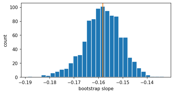
Estimate the SE of the slope of mpg ~ horsepower.

from sklearn.linear_model import LinearRegression
B = 1000
boots = np.empty(B)
n = len(X)
for b in range(B):
    idx = rng.integers(0, n, size=n)
    boots[b] = LinearRegression().fit(X[idx], y[idx]).coef_[0]
print('bootstrap SE      :', boots.std(ddof=1).round(4))
print('bootstrap 95% CI  :', np.quantile(boots, [0.025, 0.975]).round(4))
import statsmodels.api as sm
Xc = sm.add_constant(X)
ols = sm.OLS(y, Xc).fit()
print('OLS SE            :', round(ols.bse[1], 4))
print('OLS 95% CI        :', ols.conf_int().iloc[1].round(4).tolist()
    if hasattr(ols.conf_int(), 'iloc') else ols.conf_int()[1].round(4).tolist())

bootstrap SE      : 0.0077
bootstrap 95% CI  : [-0.1754 -0.1439]
OLS SE            : 0.0064
OLS 95% CI        : [-0.1705, -0.1452]

Plot the bootstrap distribution.

fig, ax = plt.subplots(figsize=(6, 3))
ax.hist(boots, bins=30, edgecolor='white')
ax.axvline(boots.mean(), color='C1')
ax.set(xlabel='bootstrap slope', ylabel='count'); plt.show()

../_images/c36fd967dc4c685609a2ab1cca711033abdfef59360160d6a7a768e0315867f0.png

Lecture exercises — worked Python solutions¶

The cells below mirror the [Python]-tagged exercises from the Chapter 5 lecture slides, with fully worked, runnable solutions and the expected numeric answers (stored as inline comments). Each solution uses the load() helper from the setup cell, so it runs locally or on Colab with no hard-coded paths.

Exercise 5.6 — Bootstrap SE of the Portfolio $\alpha$¶

The Portfolio data has two return series X and Y. The minimum-variance allocation to asset X is $$\hat\alpha=\frac{\hat\sigma_Y^2-\hat\sigma_{XY}}{\hat\sigma_X^2+\hat\sigma_Y^2-2\hat\sigma_{XY}}.$$ Compute $\hat\alpha$ on the full sample and estimate its standard error with $B=1000$ bootstrap resamples (rows drawn *with replacement*, keeping each $(X_i,Y_i)$ pair together).

# Exercise 5.6 -- bootstrap standard error of the Portfolio allocation alpha.
# alpha is a nonlinear ratio of variances/covariance, so no closed-form SE
# exists -> the bootstrap is the natural tool (ISLP Section 5.2).
Port   = load('Portfolio')                       # columns X, Y (asset returns)
Xp, Yp = Port['X'].values, Port['Y'].values

def alpha_hat(x, y):                             # minimum-variance allocation
    sx, sy = np.var(x, ddof=1), np.var(y, ddof=1)    # sample variances
    sxy    = np.cov(x, y, ddof=1)[0, 1]              # sample covariance
    return (sy - sxy) / (sx + sy - 2 * sxy)

rng  = np.random.default_rng(0)                  # reproducible (matches slide)
n, B = len(Xp), 1000                             # B bootstrap replications
reps = np.empty(B)
for b in range(B):
    idx     = rng.integers(0, n, size=n)         # ONE shared index -> keep pairs
    reps[b] = alpha_hat(Xp[idx], Yp[idx])        # recompute alpha on the resample

print('alpha_hat    :', round(alpha_hat(Xp, Yp), 4))   # 0.5758  (~0.58)
print('bootstrap SE :', round(reps.std(ddof=1), 4))    # 0.0912  (~0.09)

alpha_hat    : 0.5758
bootstrap SE : 0.0912

Interpretation. The point estimate is $\hat\alpha\approx0.58$ with a bootstrap standard error of $\approx0.09$, matching ISLP Section 5.2: across resamples the estimated optimal allocation to asset X varies by about $\pm0.09$ — an uncertainty statement that no closed-form formula supplies for $\alpha$. Common mistake: drawing separate index vectors for X and Y, which destroys the $X$–$Y$ covariance the statistic depends on; one shared idx keeps the pairs intact.

Extended Exercise 5.2 — Bootstrap SE: statistic and coefficient¶

Extend Exercise 5.6 in two directions: (1) report a 95% percentile confidence interval for the Portfolio $\hat\alpha$ alongside its bootstrap SE; and (2) bootstrap the OLS slope of mpg on horsepower in the Auto data and compare the bootstrap SE with the textbook (formula-based) OLS standard error.

# Extended Exercise 5.2 -- (1) percentile CI for alpha, (2) bootstrap the OLS
# slope and compare it with the formula-based SE.  Reuses alpha_hat, Xp, Yp, n
# defined in Exercise 5.6 above.
import statsmodels.api as sm

# --- (1) Portfolio alpha: bootstrap SE + 95% percentile interval ----------
rng  = np.random.default_rng(0)                  # reproducible (matches slide)
reps = np.empty(1000)
for b in range(1000):
    idx     = rng.integers(0, n, size=n)         # one shared index -> keep pairs
    reps[b] = alpha_hat(Xp[idx], Yp[idx])
print('alpha_hat        :', round(alpha_hat(Xp, Yp), 4))                    # 0.5758
print('alpha SE         :', round(reps.std(ddof=1), 4))                     # 0.0912
print('alpha 95% pctile :', np.round(np.quantile(reps, [.025, .975]), 3))  # [0.413 0.77]

# --- (2) Auto: bootstrap OLS slope vs formula-based SE --------------------
Auto = load('Auto', na_values='?').dropna()
hp   = Auto['horsepower'].values.astype(float)   # predictor
mpg  = Auto['mpg'].values                        # response
ols  = sm.OLS(mpg, sm.add_constant(hp)).fit()    # single fit -> formula SE
print('OLS slope        :', round(ols.params[1], 4))    # -0.1578
print('OLS formula SE   :', round(ols.bse[1], 5))       #  0.00645

rng    = np.random.default_rng(0)
m      = len(hp)
slopes = np.empty(1000)
for b in range(1000):
    idx       = rng.integers(0, m, size=m)       # resample rows with replacement
    slopes[b] = sm.OLS(mpg[idx], sm.add_constant(hp[idx])).fit().params[1]
print('bootstrap SE     :', round(slopes.std(ddof=1), 5))                     # 0.00746
print('bootstrap 95% CI :', np.round(np.quantile(slopes, [.025, .975]), 4))   # [-0.1732 -0.1443]

alpha_hat        : 0.5758
alpha SE         : 0.0912
alpha 95% pctile : [0.413 0.77 ]
OLS slope        : -0.1578
OLS formula SE   : 0.00645
bootstrap SE     : 0.00746
bootstrap 95% CI : [-0.1732 -0.1443]

Interpretation. The Portfolio 95% percentile interval $\approx[0.41,\,0.77]$ turns the point estimate into an honest uncertainty range. For the Auto slope, the bootstrap SE ($\approx0.0075$) is close to the OLS formula SE ($\approx0.0064$), which validates the bootstrap. Where they differ the bootstrap is often more trustworthy: the formula SE assumes a correctly specified linear model with constant-variance errors, whereas the bootstrap assumes neither and picks up the mild nonlinearity/heteroscedasticity in Auto — hence the slightly larger bootstrap SE.

6. Exercises¶

Bootstrap the intercept and compare to the OLS SE.
Repeat the polynomial CV using weight instead of horsepower. Which degree wins?
Write a function boot_stat(data, stat, B=1000) that returns $B$ bootstrap replications of stat(data).
Use the bootstrap to estimate the SE of the minimum of a Gaussian sample. Compare with the parametric formula.