
This notebook runs on Colab as-is. The badge link above and the GITHUB_RAW line in the setup cell already point to this repository, so everything installs and loads automatically.
Chapter 13 — Multiple Testing
Lab: Bonferroni, Holm, Benjamini–Hochberg, permutation tests
Course: Quantitative Research Methods
Instructor: Prof. Dr. Christoph Weisser, HSBI
Source: James, Witten, Hastie, Tibshirani & Taylor (2023), An Introduction to Statistical Learning, with Applications in Python, Springer. Companion code at statlearning.com.
Goal. Run a multiple-testing simulation; compare FWER- and FDR-controlling procedures; build a permutation \(p\)-value.
Setup
Run this cell once. The ISLP package can be installed with pip install ISLP. As an alternative, the same data sets are available as CSVs in the workspace’s ALL CSV FILES - 2nd Edition folder.
Google Colab: this notebook also runs on Colab out of the box — the setup cell below installs any missing packages and downloads the data automatically.
# --- Setup: runs locally AND on Google Colab --------------------------------
# Silence only the spurious 'encountered in matmul' RuntimeWarnings that the macOS
# Accelerate BLAS emits; real warnings (deprecations, model caveats) stay visible.
import warnings
warnings.filterwarnings('ignore', message='.*encountered in matmul', category=RuntimeWarning)
import importlib.util, os, subprocess, sys

IN_COLAB = 'google.colab' in sys.modules

def _ensure(pkg, import_name=None):
    """pip-install pkg (quietly) if its import is missing."""
    if importlib.util.find_spec(import_name or pkg) is None:
        subprocess.run([sys.executable, '-m', 'pip', 'install', '-q', pkg], check=False)

if IN_COLAB:  # Colab ships numpy/pandas/sklearn/statsmodels; add course extras
    for _pkg, _imp in [('ISLP', 'ISLP')]:
        _ensure(_pkg, _imp)

import numpy as np
import pandas as pd
import matplotlib.pyplot as plt

rng = np.random.default_rng(2024)
plt.rcParams['figure.dpi'] = 110

try:
    from ISLP import load_data
    HAVE_ISLP = True
except ImportError:
    HAVE_ISLP = False
    print('ISLP not installed; using CSV / URL fallbacks.')

# Local CSV location (repo layout first, then legacy paths, then a data/ cache).
_CANDIDATES = ['../ALL CSV FILES - 2nd Edition',
               'ALL CSV FILES - 2nd Edition',
               '../../ALL CSV FILES - 2nd Edition', 'data']
CSV = next((p for p in _CANDIDATES if os.path.isdir(p)), 'data')

# GITHUB_RAW lets a fresh Colab runtime fetch any
# CSV that is neither in ISLP nor already local (spaces in the folder -> %20).
GITHUB_RAW = ('https://raw.githubusercontent.com/ChrisW09/Quantitative-Research-Methods/main/'
              'ALL%20CSV%20FILES%20-%202nd%20Edition')

# The four datasets NOT in the ISLP package -> load from the book's official
# site so the notebook works on a fresh Colab even before the repo is published.
KNOWN_URLS = {
    'Advertising': 'https://www.statlearning.com/s/Advertising.csv',
    'Heart':       'https://www.statlearning.com/s/Heart.csv',
    'Income1':     'https://www.statlearning.com/s/Income1.csv',
    'Income2':     'https://www.statlearning.com/s/Income2.csv',
}

def load(name, **read_csv_kwargs):
    """Load a course dataset. Order: ISLP package -> R datasets -> local CSV
    -> official book URL -> your GitHub repo. Works locally and on Colab."""
    if HAVE_ISLP:
        try:
            return load_data(name)
        except Exception:
            pass
    if name == 'USArrests':                       # classic R dataset, not in ISLP
        try:
            import statsmodels.api as sm
            return sm.datasets.get_rdataset('USArrests', 'datasets').data
        except Exception:
            pass
    path = f'{CSV}/{name}.csv'
    if os.path.exists(path):                      # running from the repo (local)
        return pd.read_csv(path, **read_csv_kwargs)
    remotes = ([KNOWN_URLS[name]] if name in KNOWN_URLS else []) + [f'{GITHUB_RAW}/{name}.csv']
    for url in remotes:                           # fresh Colab: stream over https
        try:
            return pd.read_csv(url, **read_csv_kwargs)
        except Exception:
            continue
    raise FileNotFoundError(
        f"Could not load {name!r}. Put the CSV in '{CSV}/' or check your connection for the GITHUB_RAW fallback.")
1. Simulation: \(m = 1000\) tests, \(5\,\%\) true alternatives
from scipy.stats import ttest_1samp
from statsmodels.stats.multitest import multipletests

m, n_true, n = 1000, 50, 30
X = rng.standard_normal(size=(n, m))
true_mean = np.zeros(m)
true_mean[:n_true] = 0.6
X = X + true_mean
p = np.array([ttest_1samp(X[:, j], 0).pvalue for j in range(m)])
print('first 10 p-values:', np.round(p[:10], 3))
first 10 p-values: [0.432 0.003 0.019 0. 0.106 0. 0. 0.086 0.067 0.001]
2. Compare procedures
for method in ['bonferroni', 'holm', 'fdr_bh']:
    rej, p_corr, *_ = multipletests(p, alpha=0.05, method=method)
    tp = rej[:n_true].sum(); fp = rej[n_true:].sum()
    fdr = fp / max(rej.sum(), 1)
    print(f'{method:11s}  rejected={rej.sum():3d}  TP={tp:3d}  FP={fp:3d}  realised FDP={fdr:.3f}')
bonferroni   rejected=  7  TP=  7  FP=  0  realised FDP=0.000
holm         rejected=  7  TP=  7  FP=  0  realised FDP=0.000
fdr_bh       rejected= 23  TP= 20  FP=  3  realised FDP=0.130
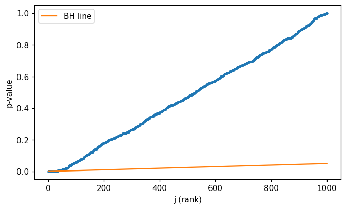
3. Visualise the Benjamini-Hochberg line
p_sorted = np.sort(p)
j = np.arange(1, m + 1)
q = 0.05
fig, ax = plt.subplots(figsize=(7, 4))
ax.scatter(j, p_sorted, s=4)
ax.plot(j, j * q / m, color='C1', label='BH line')
ax.set(xlabel='j (rank)', ylabel='p-value'); ax.legend()
plt.show()
4. Permutation test
def perm_pvalue(x, B=2000, rng=rng):
    obs = np.abs(x.mean())
    n = len(x)
    null = np.array([
        np.abs((rng.choice([-1, 1], size=n) * x).mean()) for _ in range(B)
    ])
    return (null >= obs).mean()

z = rng.standard_normal(40) + 0.5
print('permutation p-value:', perm_pvalue(z))
from scipy.stats import ttest_1samp
print('parametric  p-value:', ttest_1samp(z, 0).pvalue)
permutation p-value: 0.0065
parametric  p-value: 0.0076141250910252
Lecture exercises — worked Python solutions
These are the [Python]-tagged exercises from the lecture slides, solved step by step. Run each cell and compare with the slide solutions.
Extended Exercise 13.3 — Simulating FDR and power [Python]
Simulate m=1000 one-sided z-tests, m1=100 with a true effect (mean shift mu=3). Over ~2000 repeats, apply Benjamini–Hochberg at q=0.10 and Bonferroni at alpha=0.05, and estimate the realised FDR (V/R) and power (S/m1).
import numpy as np                 # arrays and random numbers
from scipy import stats            # normal cdf for p-values

rng = np.random.default_rng(0)     # seeded generator: reproducible
m, m1, mu = 1000, 100, 3.0         # 100 true effects, mean shift mu
q, alpha  = 0.10, 0.05             # FDR target q, FWER target alpha
truth = np.arange(m) < m1          # first m1 tests are non-null

def bh_reject(p, q):               # Benjamini-Hochberg step-up procedure
    order = np.argsort(p); ps = p[order]        # sort p-values ascending
    thr = (np.arange(1, m + 1) / m) * q         # BH line: (j/m) * q
    hit = np.where(ps <= thr)[0]                # ranks below the line
    rej = np.zeros(m, bool)                     # start: reject nothing
    if len(hit):
        rej[order[:hit.max() + 1]] = True       # reject up to the largest hit
    return rej

def simulate(method, reps=2000):               # average FDR / power over reps
    fdr = pw = 0.0
    for _ in range(reps):
        z = rng.normal(0, 1, m)                 # null z-scores
        z[:m1] = rng.normal(mu, 1, m1)          # inject the true effects
        p = 1 - stats.norm.cdf(z)               # one-sided p-values
        rej = bh_reject(p, q) if method == "bh" else (p <= alpha / m)
        V = (rej & ~truth).sum()                # false rejections
        S = (rej &  truth).sum()                # true rejections
        R = rej.sum()                           # total rejections
        fdr += V / max(R, 1); pw += S / m1      # realised FDP and power
    return fdr / reps, pw / reps

for meth in ["bh", "bonferroni"]:
    f, pw = simulate(meth)          # pw, not p: p holds the earlier p-values
    print("%-11s FDR=%.3f power=%.3f" % (meth, f, pw))
print("BH theoretical bound q*m0/m =", q * (m - m1) / m)
# Expected: bh FDR=0.090 power=0.723 ; bonferroni FDR=0.002 power=0.186 ; bound=0.09
bh          FDR=0.090 power=0.723
bonferroni  FDR=0.002 power=0.186
BH theoretical bound q*m0/m = 0.09
Reading the output. BH holds the realised FDR right at its bound q·m0/m = 0.09 while recovering ~72% of the true effects. Bonferroni is far stricter (FDR ≈ 0.002) but pays for it in power (~19%): controlling the probability of any false positive is much more conservative than controlling the fraction of them.
5. Exercises
Increase \(m\) to 10 000 and re-run. How does power change?
Replace
0.6with0.3(smaller effect) and observe how FDR and power respond.Implement Storey’s \(\hat\pi_0\) estimator and the resulting \(q\)-values.
Use a permutation test to compare two-sample means; compare with the parametric \(t\)-test under non-Gaussian data.