
This notebook runs on Colab as-is. The badge link above and the GITHUB_RAW line in the setup cell already point to this repository, so everything installs and loads automatically.
Chapter 6 — Model Selection and Regularisation
Lab: subset selection, ridge, lasso, PCR, PLS
Course: Quantitative Research Methods
Instructor: Prof. Dr. Christoph Weisser, HSBI
Source: James, Witten, Hastie, Tibshirani & Taylor (2023), An Introduction to Statistical Learning, with Applications in Python, Springer. Companion code at statlearning.com.
Goal. On the Hitters data, fit best-subset, ridge, lasso, PCR, and PLS, and compare them by cross-validation.
Setup
Run this cell once. The ISLP package can be installed with pip install ISLP. As an alternative, the same data sets are available as CSVs in the workspace’s ALL CSV FILES - 2nd Edition folder.
Google Colab: this notebook also runs on Colab out of the box — the setup cell below installs any missing packages and downloads the data automatically.
# --- Setup: runs locally AND on Google Colab --------------------------------
# Silence only the spurious 'encountered in matmul' RuntimeWarnings that the macOS
# Accelerate BLAS emits; real warnings (deprecations, model caveats) stay visible.
import warnings
warnings.filterwarnings('ignore', message='.*encountered in matmul', category=RuntimeWarning)
import importlib.util, os, subprocess, sys

IN_COLAB = 'google.colab' in sys.modules

def _ensure(pkg, import_name=None):
    """pip-install pkg (quietly) if its import is missing."""
    if importlib.util.find_spec(import_name or pkg) is None:
        subprocess.run([sys.executable, '-m', 'pip', 'install', '-q', pkg], check=False)

if IN_COLAB:  # Colab ships numpy/pandas/sklearn/statsmodels; add course extras
    for _pkg, _imp in [('ISLP', 'ISLP')]:
        _ensure(_pkg, _imp)

import numpy as np
import pandas as pd
import matplotlib.pyplot as plt

rng = np.random.default_rng(2024)
plt.rcParams['figure.dpi'] = 110

try:
    from ISLP import load_data
    HAVE_ISLP = True
except ImportError:
    HAVE_ISLP = False
    print('ISLP not installed; using CSV / URL fallbacks.')

# Local CSV location (repo layout first, then legacy paths, then a data/ cache).
_CANDIDATES = ['../ALL CSV FILES - 2nd Edition',
               'ALL CSV FILES - 2nd Edition',
               '../../ALL CSV FILES - 2nd Edition', 'data']
CSV = next((p for p in _CANDIDATES if os.path.isdir(p)), 'data')

# GITHUB_RAW lets a fresh Colab runtime fetch any
# CSV that is neither in ISLP nor already local (spaces in the folder -> %20).
GITHUB_RAW = ('https://raw.githubusercontent.com/ChrisW09/Quantitative-Research-Methods/main/'
              'ALL%20CSV%20FILES%20-%202nd%20Edition')

# The four datasets NOT in the ISLP package -> load from the book's official
# site so the notebook works on a fresh Colab even before the repo is published.
KNOWN_URLS = {
    'Advertising': 'https://www.statlearning.com/s/Advertising.csv',
    'Heart':       'https://www.statlearning.com/s/Heart.csv',
    'Income1':     'https://www.statlearning.com/s/Income1.csv',
    'Income2':     'https://www.statlearning.com/s/Income2.csv',
}

def load(name, **read_csv_kwargs):
    """Load a course dataset. Order: ISLP package -> R datasets -> local CSV
    -> official book URL -> your GitHub repo. Works locally and on Colab."""
    if HAVE_ISLP:
        try:
            return load_data(name)
        except Exception:
            pass
    if name == 'USArrests':                       # classic R dataset, not in ISLP
        try:
            import statsmodels.api as sm
            return sm.datasets.get_rdataset('USArrests', 'datasets').data
        except Exception:
            pass
    path = f'{CSV}/{name}.csv'
    if os.path.exists(path):                      # running from the repo (local)
        return pd.read_csv(path, **read_csv_kwargs)
    remotes = ([KNOWN_URLS[name]] if name in KNOWN_URLS else []) + [f'{GITHUB_RAW}/{name}.csv']
    for url in remotes:                           # fresh Colab: stream over https
        try:
            return pd.read_csv(url, **read_csv_kwargs)
        except Exception:
            continue
    raise FileNotFoundError(
        f"Could not load {name!r}. Put the CSV in '{CSV}/' or check your connection for the GITHUB_RAW fallback.")
1. Hitters data
Hitters = load('Hitters').dropna().reset_index(drop=True)
y = Hitters['Salary']
X = Hitters.drop(columns='Salary')
X = pd.get_dummies(X, drop_first=True).astype(float)
print(X.shape); X.head()
(263, 19)
| AtBat | Hits | HmRun | Runs | RBI | Walks | Years | CAtBat | CHits | CHmRun | CRuns | CRBI | CWalks | PutOuts | Assists | Errors | League_N | Division_W | NewLeague_N | |
|---|---|---|---|---|---|---|---|---|---|---|---|---|---|---|---|---|---|---|---|
| 0 | 315.0 | 81.0 | 7.0 | 24.0 | 38.0 | 39.0 | 14.0 | 3449.0 | 835.0 | 69.0 | 321.0 | 414.0 | 375.0 | 632.0 | 43.0 | 10.0 | 1.0 | 1.0 | 1.0 |
| 1 | 479.0 | 130.0 | 18.0 | 66.0 | 72.0 | 76.0 | 3.0 | 1624.0 | 457.0 | 63.0 | 224.0 | 266.0 | 263.0 | 880.0 | 82.0 | 14.0 | 0.0 | 1.0 | 0.0 |
| 2 | 496.0 | 141.0 | 20.0 | 65.0 | 78.0 | 37.0 | 11.0 | 5628.0 | 1575.0 | 225.0 | 828.0 | 838.0 | 354.0 | 200.0 | 11.0 | 3.0 | 1.0 | 0.0 | 1.0 |
| 3 | 321.0 | 87.0 | 10.0 | 39.0 | 42.0 | 30.0 | 2.0 | 396.0 | 101.0 | 12.0 | 48.0 | 46.0 | 33.0 | 805.0 | 40.0 | 4.0 | 1.0 | 0.0 | 1.0 |
| 4 | 594.0 | 169.0 | 4.0 | 74.0 | 51.0 | 35.0 | 11.0 | 4408.0 | 1133.0 | 19.0 | 501.0 | 336.0 | 194.0 | 282.0 | 421.0 | 25.0 | 0.0 | 1.0 | 0.0 |
2. Best-subset and forward stepwise selection
Brute-force best-subset for small \(k\); forward stepwise for comparability.
import itertools, statsmodels.api as sm
from sklearn.metrics import mean_squared_error
preds = X.columns.tolist()
best = {}
for k in range(1, 6):
    best_rss, best_combo = None, None
    for combo in itertools.combinations(preds, k):
        rss = sm.OLS(y, sm.add_constant(X[list(combo)])).fit().ssr
        if best_rss is None or rss < best_rss:
            best_rss, best_combo = rss, combo
    best[k] = best_combo
best
{1: ('CRBI',),
 2: ('Hits', 'CRBI'),
 3: ('Hits', 'CRBI', 'PutOuts'),
 4: ('Hits', 'CRBI', 'PutOuts', 'Division_W'),
 5: ('AtBat', 'Hits', 'CRBI', 'PutOuts', 'Division_W')}
# Forward stepwise
remaining = preds.copy(); selected = []
for step in range(8):
    best_rss, best_v = None, None
    for v in remaining:
        rss = sm.OLS(y, sm.add_constant(X[selected + [v]])).fit().ssr
        if best_rss is None or rss < best_rss:
            best_rss, best_v = rss, v
    selected.append(best_v); remaining.remove(best_v)
    print(step + 1, '->', selected[-1], 'RSS =', round(best_rss, 1))
1 -> CRBI RSS = 36179679.3
2 -> Hits RSS = 30646559.9
3 -> PutOuts RSS = 29249296.9
4 -> Division_W RSS = 27970851.8
5 -> AtBat RSS = 27149899.4
6 -> Walks RSS = 26194903.9
7 -> CWalks RSS = 25954217.1
8 -> CRuns RSS = 25159233.9
3. Ridge regression
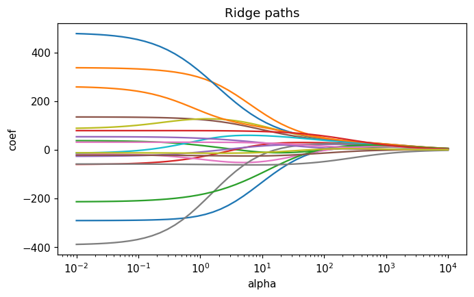
Here and for the lasso below, the penalty is selected with the scaler nested inside the search: standardising all 263 rows first and only then letting RidgeCV/LassoCV split would score every candidate \(\lambda\) on data whose means and standard deviations were computed with help from the very rows being held out.
from sklearn.linear_model import Ridge
from sklearn.preprocessing import StandardScaler
from sklearn.pipeline import make_pipeline
from sklearn.model_selection import GridSearchCV, LeaveOneOut
alphas = np.logspace(-2, 4, 50)
ridge_cv = GridSearchCV(make_pipeline(StandardScaler(), Ridge()),  # scaler per fold
                        {'ridge__alpha': alphas},
                        cv=LeaveOneOut(),      # RidgeCV's own default is leave-one-out
                        scoring='neg_mean_squared_error').fit(X, y)
ridge = ridge_cv.best_estimator_.named_steps['ridge']
print('best alpha:', ridge_cv.best_params_['ridge__alpha'])
print(pd.Series(ridge.coef_, index=X.columns).round(2))
best alpha: 2.8117686979742307
AtBat         -229.01
Hits           245.55
HmRun            4.61
Runs            -5.48
RBI              2.44
Walks          110.78
Years          -50.10
CAtBat        -115.25
CHits          123.26
CHmRun          56.29
CRuns          220.11
CRBI           120.98
CWalks        -154.21
PutOuts         77.87
Assists         40.90
Errors         -24.92
League_N        30.46
Division_W     -61.51
NewLeague_N    -13.75
dtype: float64
Ridge coefficient paths
from sklearn.linear_model import Ridge
Xs = StandardScaler().fit_transform(X)
paths = np.array([Ridge(alpha=a).fit(Xs, y).coef_ for a in alphas])
fig, ax = plt.subplots(figsize=(7, 4))
for j, name in enumerate(X.columns):
    ax.plot(alphas, paths[:, j], label=name)
ax.set_xscale('log'); ax.set_xlabel('alpha'); ax.set_ylabel('coef')
ax.set_title('Ridge paths'); plt.show()
4. Lasso
from sklearn.linear_model import Lasso
alphas = np.logspace(-3, 2, 50)
lasso_cv = GridSearchCV(make_pipeline(StandardScaler(), Lasso(max_iter=100000)),
                        {'lasso__alpha': alphas},   # scaler re-fit on each of the 10 folds
                        cv=10, scoring='neg_mean_squared_error').fit(X, y)
lasso = lasso_cv.best_estimator_.named_steps['lasso']
print('best alpha:', lasso_cv.best_params_['lasso__alpha'])
coefs = pd.Series(lasso.coef_, index=X.columns)
print('non-zero:', coefs[coefs != 0].round(2))
best alpha: 2.329951810515372
non-zero: AtBat        -243.56
Hits          266.12
HmRun           0.03
Walks         106.57
Years         -47.64
CHmRun         47.06
CRuns         230.24
CRBI          122.30
CWalks       -150.86
PutOuts        76.96
Assists        27.85
Errors        -14.46
League_N       16.38
Division_W    -59.59
dtype: float64
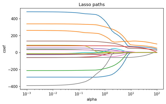
Lasso paths
Xs = StandardScaler().fit_transform(X)
paths = np.array([Lasso(alpha=a, max_iter=10000).fit(Xs, y).coef_ for a in alphas])
fig, ax = plt.subplots(figsize=(7, 4))
for j in range(paths.shape[1]):
    ax.plot(alphas, paths[:, j])
ax.set_xscale('log'); ax.set_xlabel('alpha'); ax.set_ylabel('coef')
ax.set_title('Lasso paths'); plt.show()
5. PCR and PLS
from sklearn.decomposition import PCA
from sklearn.cross_decomposition import PLSRegression
from sklearn.linear_model import LinearRegression
from sklearn.model_selection import cross_val_score
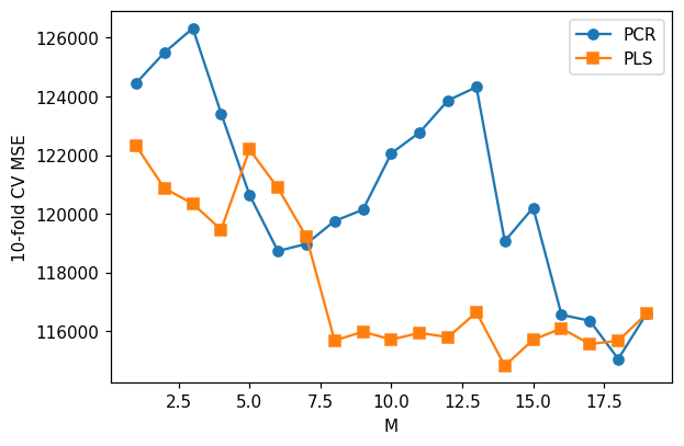
# StandardScaler is a step *inside* each pipeline, so cross_val_score re-fits it
# on every training fold; standardising X once up front would let each held-out
# fold help set the means and standard deviations used to train.
pcr_scores = []; pls_scores = []
for M in range(1, X.shape[1] + 1):
    pcr = make_pipeline(StandardScaler(), PCA(n_components=M), LinearRegression())
    pls = make_pipeline(StandardScaler(), PLSRegression(n_components=M, scale=False))
    pcr_scores.append(-cross_val_score(pcr, X, y, cv=10,
                                         scoring='neg_mean_squared_error').mean())
    pls_scores.append(-cross_val_score(pls, X, y, cv=10,
                                         scoring='neg_mean_squared_error').mean())
fig, ax = plt.subplots(figsize=(6, 4))
Ms = range(1, X.shape[1] + 1)
ax.plot(Ms, pcr_scores, marker='o', label='PCR')
ax.plot(Ms, pls_scores, marker='s', label='PLS')
ax.set(xlabel='M', ylabel='10-fold CV MSE'); ax.legend(); plt.show()
Lecture exercises — worked Python solutions
The cells below mirror the [Python]-tagged exercises from the Chapter 6 lecture slides, with fully worked, runnable solutions and the expected numeric answers (stored as inline comments). Each solution reloads Hitters through the load() helper so it stands alone and reproduces the slide numbers.
Exercise 6.7 — CV ridge and lasso on Hitters
On the Hitters data (predict Salary): (i) fit the lasso with a cross-validated \(\lambda\) on standardised predictors, (ii) report the selected \(\lambda\), and (iii) list which features the lasso keeps versus drops. Contrast with ridge, which keeps every predictor.
# Exercise 6.7 -- lasso vs ridge with a cross-validated penalty on Hitters.
from sklearn.linear_model    import Lasso, Ridge
from sklearn.preprocessing   import StandardScaler
from sklearn.pipeline        import make_pipeline
from sklearn.model_selection import GridSearchCV

df    = load('Hitters').dropna()                 # drop the 59 rows with NA Salary
yH    = df['Salary'].values
X_raw = pd.get_dummies(df.drop(columns='Salary'),    # encode League/Division/NewLeague
                       drop_first=True).astype(float)
preds = X_raw.columns
print('n, p =', X_raw.shape)                     # (263, 19)

# Standardising matters (the penalty is scale-dependent), but it has to happen
# INSIDE the pipeline: GridSearchCV then re-fits the scaler on each training
# fold, so no validation fold ever helps set the scaling used to train.
lasso_cv = GridSearchCV(make_pipeline(StandardScaler(), Lasso(max_iter=100000)),
                        {'lasso__alpha': np.logspace(-3, 2, 50)},
                        cv=10, scoring='neg_mean_squared_error').fit(X_raw, yH)
lasso = lasso_cv.best_estimator_.named_steps['lasso']            # CV lambda
print('lasso alpha :', round(lasso_cv.best_params_['lasso__alpha'], 3))   # 2.33
kept    = [p for p, c in zip(preds, lasso.coef_) if abs(c) >  1e-8]
dropped = [p for p, c in zip(preds, lasso.coef_) if abs(c) <= 1e-8]
print('kept    :', kept)      # Hits, Walks, CRBI, PutOuts, Division_W, ...
print('dropped :', dropped)   # Runs, RBI, CAtBat, CHits, NewLeague_N

ridge_cv = GridSearchCV(make_pipeline(StandardScaler(), Ridge()),   # same recipe
                        {'ridge__alpha': np.logspace(-2, 4, 50)},
                        cv=10, scoring='neg_mean_squared_error').fit(X_raw, yH)
ridge = ridge_cv.best_estimator_.named_steps['ridge']
print('ridge alpha :', round(ridge_cv.best_params_['ridge__alpha'], 3),
      '-- nonzero coefs:', int(np.sum(np.abs(ridge.coef_) > 1e-8)))   # 2.812 -- 19
n, p = (263, 19)
lasso alpha : 2.33
kept    : ['AtBat', 'Hits', 'HmRun', 'Walks', 'Years', 'CHmRun', 'CRuns', 'CRBI', 'CWalks', 'PutOuts', 'Assists', 'Errors', 'League_N', 'Division_W']
dropped : ['Runs', 'RBI', 'CAtBat', 'CHits', 'NewLeague_N']
ridge alpha : 2.812 -- nonzero coefs: 19
Interpretation. The lasso selects a moderate \(\lambda\approx2.33\) and drives several coefficients exactly to zero — it keeps strong career/recent-performance predictors (e.g. Hits, Walks, CRBI, PutOuts, Division_W) and drops weak or redundant ones (Runs, RBI, CAtBat, CHits, NewLeague_N). Ridge keeps all 19 predictors nonzero (it only shrinks). Takeaway: the lasso yields a sparse, more interpretable model via automatic variable selection, whereas ridge stabilises the fit while retaining every predictor. Note where the standardisation lives: it is a pipeline step that GridSearchCV re-fits on every training fold, because a scaler fitted once on the whole matrix has already seen each validation fold — the leakage the Chapter 5 lab warns about.
Extended Exercise 6.3 — CV ridge and lasso test MSE on Hitters
Split Hitters into train/test, standardise using the training set only (no leakage), and cross-validate \(\lambda\) for both ridge and lasso. Report each chosen \(\lambda\), the test MSE, and how many coefficients are non-zero; list the predictors the lasso drops.
# Extended Exercise 6.3 -- honest test-MSE comparison with leak-free scaling.
from sklearn.model_selection import train_test_split
from sklearn.preprocessing   import StandardScaler
from sklearn.linear_model    import RidgeCV, LassoCV
from sklearn.metrics         import mean_squared_error

df  = load('Hitters').dropna(subset=['Salary'])  # drop rows with NA response
yH  = df['Salary'].values
XH  = pd.get_dummies(df.drop(columns='Salary'),
                     drop_first=True).astype(float)
Xtr, Xte, ytr, yte = train_test_split(XH.values, yH,
                        test_size=0.33, random_state=1)    # 2/3 - 1/3 split
sc = StandardScaler().fit(Xtr)                   # fit scaler on TRAIN only
Xtr, Xte = sc.transform(Xtr), sc.transform(Xte)  # apply to both -> no leakage

ridge = RidgeCV(alphas=np.logspace(-2, 4, 50)).fit(Xtr, ytr)
lasso = LassoCV(cv=10, max_iter=100000, random_state=0).fit(Xtr, ytr)
for name, m in [('ridge', ridge), ('lasso', lasso)]:
    mse = mean_squared_error(yte, m.predict(Xte))        # TEST-set MSE
    nz  = int(np.sum(np.abs(m.coef_) > 1e-8))            # nonzero coefficients
    print(f'{name}: lambda={round(m.alpha_, 3)}  testMSE={round(mse, 0)}  nonzero={nz}')
    # ridge: lambda=0.095  testMSE=122695.0  nonzero=19
    # lasso: lambda=0.779  testMSE=119064.0  nonzero=16
dropped = [c for c, w in zip(XH.columns, lasso.coef_) if abs(w) <= 1e-8]
print('lasso drops:', dropped)                   # ['Years', 'CRBI', 'Errors']
ridge: lambda=0.095  testMSE=122695.0  nonzero=19
lasso: lambda=0.779  testMSE=119064.0  nonzero=16
lasso drops: ['Years', 'CRBI', 'Errors']
Interpretation. With \(n=263\), \(p=19\) and this split, ridge chooses \(\lambda\approx0.1\) (test MSE \(\approx1.2\times10^5\), all 19 coefficients non-zero) while the lasso chooses \(\lambda\approx0.8\) (test MSE \(\approx1.2\times10^5\), 16 non-zero) and drops Years, CRBI, Errors (weak or redundant given the correlated career totals). Both attain nearly identical test error, but the lasso reaches it with a sparser, more interpretable model. Exact numbers shift with the split/seed; the qualitative message — lasso selects, ridge keeps all — is stable.
6. Exercises
Run backward stepwise selection and compare with forward.
Use the one-standard-error rule to choose a more parsimonious lasso \(\lambda\).
Fit elastic net on Hitters with
ElasticNetCV. How does it compare to ridge and lasso?On a high-dimensional problem (\(p > n\)), demonstrate that OLS fails while ridge / lasso work.