This notebook runs on Colab as-is. The badge link above and the GITHUB_RAW line in the setup cell already point to this repository, so everything installs and loads automatically.

Chapter 1 — Introduction

Lab: getting comfortable with the tools and the data

Course: Quantitative Research Methods
Instructor: Prof. Dr. Christoph Weisser, HSBI
Source: James, Witten, Hastie, Tibshirani & Taylor (2023), An Introduction to Statistical Learning, with Applications in Python, Springer. Companion code at statlearning.com.

Goal of this lab. Spin up the Python tooling, load the three motivating data sets (Wage, Smarket, NCI60), and reproduce the exploratory visualisations from the chapter.

Setup

Run this cell once. The ISLP package can be installed with pip install ISLP. As an alternative, the same data sets are available as CSVs in the workspace’s ALL CSV FILES - 2nd Edition folder.

Google Colab: this notebook also runs on Colab out of the box — the setup cell below installs any missing packages and downloads the data automatically.

# --- Setup: runs locally AND on Google Colab --------------------------------
# Silence only the spurious 'encountered in matmul' RuntimeWarnings that the macOS
# Accelerate BLAS emits; real warnings (deprecations, model caveats) stay visible.
import warnings
warnings.filterwarnings('ignore', message='.*encountered in matmul', category=RuntimeWarning)
import importlib.util, os, subprocess, sys

IN_COLAB = 'google.colab' in sys.modules

def _ensure(pkg, import_name=None):
    """pip-install pkg (quietly) if its import is missing."""
    if importlib.util.find_spec(import_name or pkg) is None:
        subprocess.run([sys.executable, '-m', 'pip', 'install', '-q', pkg], check=False)

if IN_COLAB:  # Colab ships numpy/pandas/sklearn/statsmodels; add course extras
    for _pkg, _imp in [('ISLP', 'ISLP')]:
        _ensure(_pkg, _imp)

import numpy as np
import pandas as pd
import matplotlib.pyplot as plt

rng = np.random.default_rng(2024)
plt.rcParams['figure.dpi'] = 110

try:
    from ISLP import load_data
    HAVE_ISLP = True
except ImportError:
    HAVE_ISLP = False
    print('ISLP not installed; using CSV / URL fallbacks.')

# Local CSV location (repo layout first, then legacy paths, then a data/ cache).
_CANDIDATES = ['../ALL CSV FILES - 2nd Edition',
               'ALL CSV FILES - 2nd Edition',
               '../../ALL CSV FILES - 2nd Edition', 'data']
CSV = next((p for p in _CANDIDATES if os.path.isdir(p)), 'data')

# GITHUB_RAW lets a fresh Colab runtime fetch any
# CSV that is neither in ISLP nor already local (spaces in the folder -> %20).
GITHUB_RAW = ('https://raw.githubusercontent.com/ChrisW09/Quantitative-Research-Methods/main/'
              'ALL%20CSV%20FILES%20-%202nd%20Edition')

# The four datasets NOT in the ISLP package -> load from the book's official
# site so the notebook works on a fresh Colab even before the repo is published.
KNOWN_URLS = {
    'Advertising': 'https://www.statlearning.com/s/Advertising.csv',
    'Heart':       'https://www.statlearning.com/s/Heart.csv',
    'Income1':     'https://www.statlearning.com/s/Income1.csv',
    'Income2':     'https://www.statlearning.com/s/Income2.csv',
}

def load(name, **read_csv_kwargs):
    """Load a course dataset. Order: ISLP package -> R datasets -> local CSV
    -> official book URL -> your GitHub repo. Works locally and on Colab."""
    if HAVE_ISLP:
        try:
            return load_data(name)
        except Exception:
            pass
    if name == 'USArrests':                       # classic R dataset, not in ISLP
        try:
            import statsmodels.api as sm
            return sm.datasets.get_rdataset('USArrests', 'datasets').data
        except Exception:
            pass
    path = f'{CSV}/{name}.csv'
    if os.path.exists(path):                      # running from the repo (local)
        return pd.read_csv(path, **read_csv_kwargs)
    remotes = ([KNOWN_URLS[name]] if name in KNOWN_URLS else []) + [f'{GITHUB_RAW}/{name}.csv']
    for url in remotes:                           # fresh Colab: stream over https
        try:
            return pd.read_csv(url, **read_csv_kwargs)
        except Exception:
            continue
    raise FileNotFoundError(
        f"Could not load {name!r}. Put the CSV in '{CSV}/' or check your connection for the GITHUB_RAW fallback.")

1. The Wage data

Survey of 3,000 men working in the central Atlantic region of the U.S. Continuous response wage \(\Rightarrow\) regression problem.

Wage = load('Wage')
print(Wage.shape)
Wage.head()

(3000, 11)

	year	age	maritl	race	education	region	jobclass	health	health_ins	logwage	wage
0	2006	18	1. Never Married	1. White	1. < HS Grad	2. Middle Atlantic	1. Industrial	1. <=Good	2. No	4.318063	75.043154
1	2004	24	1. Never Married	1. White	4. College Grad	2. Middle Atlantic	2. Information	2. >=Very Good	2. No	4.255273	70.476020
2	2003	45	2. Married	1. White	3. Some College	2. Middle Atlantic	1. Industrial	1. <=Good	1. Yes	4.875061	130.982177
3	2003	43	2. Married	3. Asian	4. College Grad	2. Middle Atlantic	2. Information	2. >=Very Good	1. Yes	5.041393	154.685293
4	2005	50	4. Divorced	1. White	2. HS Grad	2. Middle Atlantic	2. Information	1. <=Good	1. Yes	4.318063	75.043154

Wage.describe(include='all').T

	count	unique	top	freq	mean	std	min	25%	50%	75%	max
year	3000.0	NaN	NaN	NaN	2005.791	2.026167	2003.0	2004.0	2006.0	2008.0	2009.0
age	3000.0	NaN	NaN	NaN	42.414667	11.542406	18.0	33.75	42.0	51.0	80.0
maritl	3000	5	2. Married	2074	NaN	NaN	NaN	NaN	NaN	NaN	NaN
race	3000	4	1. White	2480	NaN	NaN	NaN	NaN	NaN	NaN	NaN
education	3000	5	2. HS Grad	971	NaN	NaN	NaN	NaN	NaN	NaN	NaN
region	3000	1	2. Middle Atlantic	3000	NaN	NaN	NaN	NaN	NaN	NaN	NaN
jobclass	3000	2	1. Industrial	1544	NaN	NaN	NaN	NaN	NaN	NaN	NaN
health	3000	2	2. >=Very Good	2142	NaN	NaN	NaN	NaN	NaN	NaN	NaN
health_ins	3000	2	1. Yes	2083	NaN	NaN	NaN	NaN	NaN	NaN	NaN
logwage	3000.0	NaN	NaN	NaN	4.653905	0.351753	3.0	4.447158	4.653213	4.857332	5.763128
wage	3000.0	NaN	NaN	NaN	111.703608	41.728595	20.085537	85.38394	104.921507	128.680488	318.34243

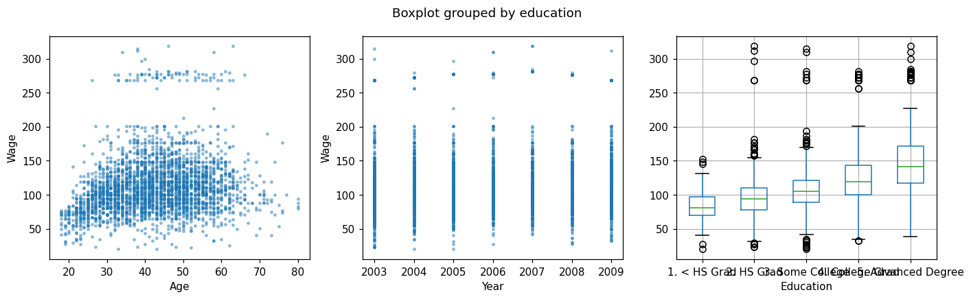
Wage vs. Age, Year, Education (Figure 1.1)

fig, axes = plt.subplots(1, 3, figsize=(13, 4))
axes[0].scatter(Wage['age'], Wage['wage'], s=5, alpha=0.4)
axes[0].set(xlabel='Age', ylabel='Wage')
axes[1].scatter(Wage['year'], Wage['wage'], s=5, alpha=0.4)
axes[1].set(xlabel='Year', ylabel='Wage')
Wage.boxplot(column='wage', by='education', ax=axes[2])
axes[2].set_title(''); axes[2].set_xlabel('Education')
plt.tight_layout(); plt.show()

Discussion

• wage increases with age then plateaus and slightly declines.

• wage rises gently with year.

• wage is sharply increasing in education.

• These suggest a non-linear dependence on age — a hint that polynomial or spline regression (Ch. 7) will help.

2. The Stock Market data

Daily S&P 500 returns from 2001–2005. Categorical response Direction \(\Rightarrow\) classification problem.

Smarket = load('Smarket')
print(Smarket.shape)
Smarket.head()

(1250, 9)

	Year	Lag1	Lag2	Lag3	Lag4	Lag5	Volume	Today	Direction
0	2001	0.381	-0.192	-2.624	-1.055	5.010	1.1913	0.959	Up
1	2001	0.959	0.381	-0.192	-2.624	-1.055	1.2965	1.032	Up
2	2001	1.032	0.959	0.381	-0.192	-2.624	1.4112	-0.623	Down
3	2001	-0.623	1.032	0.959	0.381	-0.192	1.2760	0.614	Up
4	2001	0.614	-0.623	1.032	0.959	0.381	1.2057	0.213	Up

Lag boxplots by direction (Figure 1.2)

fig, axes = plt.subplots(1, 3, figsize=(12, 4))
for ax, lag in zip(axes, ['Lag1', 'Lag2', 'Lag3']):
    Smarket.boxplot(column=lag, by='Direction', ax=ax)
    ax.set_title(lag); ax.set_xlabel('Direction')
plt.suptitle(''); plt.tight_layout(); plt.show()

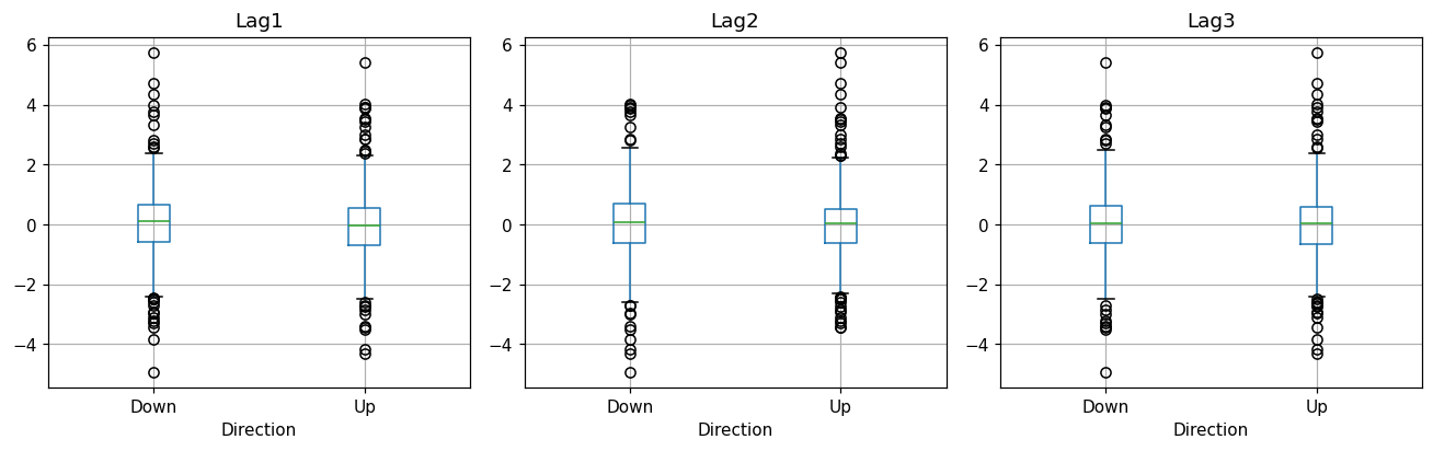
Boxplots overlap heavily — past returns barely predict the next day’s direction. Consistent with the efficient-markets view.

3. The NCI60 cancer cell lines

64 cell lines, 6 830 gene-expression measurements. No response — this is unsupervised territory.

from sklearn.preprocessing import StandardScaler
from sklearn.decomposition import PCA

if HAVE_ISLP:
    nci = load_data('NCI60')
    X = nci['data']; labs = nci['labels'].squeeze()
else:
    print('NCI60 only ships with the ISLP package.')
    X = labs = None

if X is not None:
    Xs = StandardScaler().fit_transform(X)
    Z = PCA(n_components=2).fit_transform(Xs)
    fig, ax = plt.subplots(figsize=(6, 6))
    for k in np.unique(labs):
        m = labs == k
        ax.scatter(Z[m, 0], Z[m, 1], label=k, s=18)
    ax.set_xlabel('PC 1'); ax.set_ylabel('PC 2')
    ax.legend(fontsize=7, ncol=2, loc='upper right')
    plt.show()

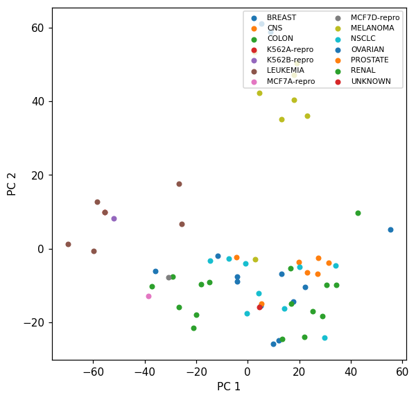
Cell lines of the same cancer type tend to cluster together — PCA recovered biologically meaningful structure without ever being told the labels.

Lecture exercises — worked Python solutions

The chapter 1 slide deck contains no [Python]-tagged exercise (its exercises are tagged [Concept], [Math], and [Integrative]). This section therefore mirrors the deck’s most code-suitable exercise — Exercise 1.3 (Notation: \(n\), \(p\), and \(\mathbf{X}\)), tagged [Math] on the slides — adapted into a fully worked, runnable Python solution. Every quantity from the slide solution is recomputed and verified in code; the expected values appear as trailing comments.

Exercise 1.3 — Notation: \(n\), \(p\), and \(\mathbf{X}\) (slide: Exercise 1.3 [Math], adapted to Python)

For five patients we record age (years), BMI, and resting heart rate HR; the response is systolic blood pressure SBP.

Patient	age	BMI	HR	SBP
1	45	24.0	70	128
2	60	29.5	82	145
3	52	26.1	75	138
4	38	22.3	68	120
5	71	31.0	90	158

1. State \(n\) and \(p\).

2. Give the dimensions of the design matrix \(\mathbf{X}\) and the response vector \(\mathbf{y}\).

3. Write the predictor vector \(x_3\) and give the value \(x_{2,3}\).

4. If an intercept column of ones is added, what are the dimensions of the model matrix?

5. Is this a regression or a classification problem?

# Exercise 1.3 — worked solution ----------------------------------------------
# The data are given in the exercise itself, so we build the table directly
# (no CSV / load() needed). Rows = observations (patients), columns = variables.
patients = pd.DataFrame(
    {'age': [45, 60, 52, 38, 71],
     'BMI': [24.0, 29.5, 26.1, 22.3, 31.0],
     'HR':  [70, 82, 75, 68, 90],
     'SBP': [128, 145, 138, 120, 158]},
    index=pd.RangeIndex(1, 6, name='patient'))

# (1) n and p. SBP is the RESPONSE we model, so it is never counted in p.
X = patients[['age', 'BMI', 'HR']].to_numpy()      # design matrix (predictors only)
y = patients['SBP'].to_numpy()                     # response vector
n, p = X.shape
print('n =', n, '  p =', p)                        # expected: n = 5   p = 3

# (2) dimensions of X and y
print('X:', X.shape, '  y:', y.shape)              # expected: X: (5, 3)   y: (5,)

# (3) x_3 = row 3 of X = all predictors of patient 3. NB: Python indexes rows
#     from 0, so slide row i is X[i - 1].
x_3 = X[3 - 1]
print('x_3  =', x_3)                               # expected: [52.  26.1 75. ]
#     x_{2,3}: FIRST index = row (observation), SECOND = column (predictor),
#     i.e. predictor 3 (HR) of patient 2 — not BMI of patient 3!
print('x_23 =', X[2 - 1, 3 - 1])                   # expected: 82.0

# (4) model matrix with an intercept column of ones prepended
X_tilde = np.column_stack([np.ones(n), X])
print('with intercept column:', X_tilde.shape)     # expected: (5, 4) = n x (p+1)

# (5) SBP is quantitative (mmHg, on a continuous scale) -> a REGRESSION problem
print('SBP dtype:', patients['SBP'].dtype, '-> quantitative -> regression')

n = 5   p = 3
X: (5, 3)   y: (5,)
x_3  = [52.  26.1 75. ]
x_23 = 82.0
with intercept column: (5, 4)
SBP dtype: int64 -> quantitative -> regression

4. Exercises

1. Reproduce the boxplots above for Lag4 and Lag5 of the Smarket data. Do you see any difference between the lags?

2. Compute the empirical correlation between wage and each numeric predictor in the Wage data set.

3. In NCI60, fit a 5-component PCA. What proportion of total variance do the first 5 components capture?

4. Pick any other ISLP data set (Boston, Auto, Default, Hitters, …), compute summary statistics, and plot the response against one continuous predictor.