This notebook runs on Colab as-is. The badge link above and the GITHUB_RAW line in the setup cell already point to this repository, so everything installs and loads automatically.

Chapter 10 — Deep Learning

Lab: training a simple MLP in PyTorch

Course: Quantitative Research Methods
Instructor: Prof. Dr. Christoph Weisser, HSBI
Source: James, Witten, Hastie, Tibshirani & Taylor (2023), An Introduction to Statistical Learning, with Applications in Python, Springer. Companion code at statlearning.com.

Goal. Build, train, and evaluate a small MLP on the Default data using PyTorch. Requires pip install torch.

Setup

Run this cell once. The ISLP package can be installed with pip install ISLP. As an alternative, the same data sets are available as CSVs in the workspace’s ALL CSV FILES - 2nd Edition folder.

Google Colab: this notebook also runs on Colab out of the box — the setup cell below installs any missing packages and downloads the data automatically.

# --- Setup: runs locally AND on Google Colab --------------------------------
# Silence only the spurious 'encountered in matmul' RuntimeWarnings that the macOS
# Accelerate BLAS emits; real warnings (deprecations, model caveats) stay visible.
import warnings
warnings.filterwarnings('ignore', message='.*encountered in matmul', category=RuntimeWarning)
import importlib.util, os, subprocess, sys

IN_COLAB = 'google.colab' in sys.modules

def _ensure(pkg, import_name=None):
    """pip-install pkg (quietly) if its import is missing."""
    if importlib.util.find_spec(import_name or pkg) is None:
        subprocess.run([sys.executable, '-m', 'pip', 'install', '-q', pkg], check=False)

if IN_COLAB:  # Colab ships numpy/pandas/sklearn/statsmodels; add course extras
    for _pkg, _imp in [('ISLP', 'ISLP'), ('torch', 'torch')]:
        _ensure(_pkg, _imp)

import numpy as np
import pandas as pd
import matplotlib.pyplot as plt

rng = np.random.default_rng(2024)
plt.rcParams['figure.dpi'] = 110

try:
    from ISLP import load_data
    HAVE_ISLP = True
except ImportError:
    HAVE_ISLP = False
    print('ISLP not installed; using CSV / URL fallbacks.')

# Local CSV location (repo layout first, then legacy paths, then a data/ cache).
_CANDIDATES = ['../ALL CSV FILES - 2nd Edition',
               'ALL CSV FILES - 2nd Edition',
               '../../ALL CSV FILES - 2nd Edition', 'data']
CSV = next((p for p in _CANDIDATES if os.path.isdir(p)), 'data')

# GITHUB_RAW lets a fresh Colab runtime fetch any
# CSV that is neither in ISLP nor already local (spaces in the folder -> %20).
GITHUB_RAW = ('https://raw.githubusercontent.com/ChrisW09/Quantitative-Research-Methods/main/'
              'ALL%20CSV%20FILES%20-%202nd%20Edition')

# The four datasets NOT in the ISLP package -> load from the book's official
# site so the notebook works on a fresh Colab even before the repo is published.
KNOWN_URLS = {
    'Advertising': 'https://www.statlearning.com/s/Advertising.csv',
    'Heart':       'https://www.statlearning.com/s/Heart.csv',
    'Income1':     'https://www.statlearning.com/s/Income1.csv',
    'Income2':     'https://www.statlearning.com/s/Income2.csv',
}

def load(name, **read_csv_kwargs):
    """Load a course dataset. Order: ISLP package -> R datasets -> local CSV
    -> official book URL -> your GitHub repo. Works locally and on Colab."""
    if HAVE_ISLP:
        try:
            return load_data(name)
        except Exception:
            pass
    if name == 'USArrests':                       # classic R dataset, not in ISLP
        try:
            import statsmodels.api as sm
            return sm.datasets.get_rdataset('USArrests', 'datasets').data
        except Exception:
            pass
    path = f'{CSV}/{name}.csv'
    if os.path.exists(path):                      # running from the repo (local)
        return pd.read_csv(path, **read_csv_kwargs)
    remotes = ([KNOWN_URLS[name]] if name in KNOWN_URLS else []) + [f'{GITHUB_RAW}/{name}.csv']
    for url in remotes:                           # fresh Colab: stream over https
        try:
            return pd.read_csv(url, **read_csv_kwargs)
        except Exception:
            continue
    raise FileNotFoundError(
        f"Could not load {name!r}. Put the CSV in '{CSV}/' or check your connection for the GITHUB_RAW fallback.")

1. Data

Default = load('Default')
Default['student_d'] = (Default['student'] == 'Yes').astype(int)
y = (Default['default'] == 'Yes').astype(int).values
X = Default[['balance', 'income', 'student_d']].values.astype('float32')
from sklearn.model_selection import train_test_split
from sklearn.preprocessing import StandardScaler
Xtr, Xte, ytr, yte = train_test_split(X, y, test_size=0.3, random_state=0)
scaler = StandardScaler().fit(Xtr)
Xtr = scaler.transform(Xtr).astype('float32')
Xte = scaler.transform(Xte).astype('float32')
print(Xtr.shape)

(7000, 3)

2. PyTorch model

try:
    import torch
    from torch import nn, optim
    from torch.utils.data import DataLoader, TensorDataset
    HAVE_TORCH = True
except Exception:
    HAVE_TORCH = False
    print('PyTorch not installed; pip install torch')

if HAVE_TORCH:
    torch.manual_seed(1)        # seed the weight init AND the loader shuffle below,
                                # so the AUC printed further down is reproducible
    class MLP(nn.Module):
        def __init__(self, p, k=32):
            super().__init__()
            self.net = nn.Sequential(
                nn.Linear(p, k), nn.ReLU(), nn.Dropout(0.2),
                nn.Linear(k, k), nn.ReLU(), nn.Dropout(0.2),
                nn.Linear(k, 2))
        def forward(self, x): return self.net(x)

    model = MLP(Xtr.shape[1])
    loss_fn = nn.CrossEntropyLoss()
    opt = optim.Adam(model.parameters(), lr=1e-3)

3. Training loop

if HAVE_TORCH:
    loader = DataLoader(
        TensorDataset(torch.tensor(Xtr), torch.tensor(ytr).long()),
        batch_size=64, shuffle=True)
    for epoch in range(40):
        for xb, yb in loader:
            opt.zero_grad()
            loss = loss_fn(model(xb), yb)
            loss.backward()
            opt.step()
    model.eval()
    with torch.no_grad():
        proba = torch.softmax(model(torch.tensor(Xte)), dim=1).numpy()[:, 1]
    from sklearn.metrics import roc_auc_score
    print('AUC:', round(roc_auc_score(yte, proba), 3))

AUC: 0.943

Lecture exercises — worked Python solutions

The [Python]-tagged exercises from the lecture slides, solved step by step. Exercise 10.6 is pure NumPy; Extended Exercise 10.3 needs a PyTorch runtime (guarded below, so the notebook still runs without torch).

Exercise 10.6 — Softmax and cross-entropy [Python]

A 3-class classifier outputs logits z = (2.0, 1.0, 0.1) for one observation whose true label is class 0. Compute the softmax probabilities and the cross-entropy loss.

import numpy as np

z = np.array([2.0, 1.0, 0.1])          # raw scores (logits)
z = z - z.max()                        # subtract max for numerical stability
p = np.exp(z) / np.exp(z).sum()        # softmax: turn logits into probabilities
ce = -np.log(p[0])                     # cross-entropy for the true class y=0
print("softmax p =", np.round(p, 3))   # -> [0.659 0.242 0.099]
print("cross-entropy =", round(ce, 3)) # -> 0.417
# The shift by z.max() does not change p (softmax is shift-invariant) but
# avoids overflow in exp(); CE = -log(prob assigned to the correct class).

softmax p = [0.659 0.242 0.099]
cross-entropy = 0.417

Reading the output. The model puts 0.659 on the correct class, so the loss −log(0.659) = 0.417 is small but non-zero. Cross-entropy only looks at the probability of the true class; it → 0 as that probability → 1 and blows up as it → 0.

Extended Exercise 10.3 — Overfitting and regularisation [Python]

Fit a PyTorch MLP to a deliberately tiny Default training set (n=200), watch it overfit, then tame it with weight decay (L2). Needs a torch runtime — runs on Colab out of the box.

try:
    import torch
    from torch import nn, optim
    HAVE_TORCH = True
except Exception:
    HAVE_TORCH = False
    print("PyTorch not installed - skipping (runs on Colab or after `pip install torch`).")

if HAVE_TORCH:
    import numpy as np
    from sklearn.preprocessing import StandardScaler
    from sklearn.model_selection import train_test_split

    Default = load("Default")                          # ISLP / local CSV / GitHub
    Default["y"]         = (Default["default"] == "Yes").astype(int)  # 0/1 response
    Default["student_d"] = (Default["student"] == "Yes").astype(int)  # dummy-code
    X = Default[["balance", "income", "student_d"]].astype(float).values
    Xtr, Xte, ytr, yte = train_test_split(
        X, Default["y"].values, train_size=200,        # deliberately tiny train set!
        random_state=0, stratify=Default["y"])
    sc = StandardScaler().fit(Xtr)                      # scale using TRAIN stats only
    Xtr, Xte = sc.transform(Xtr), sc.transform(Xte)
    Xtr, Xte = map(lambda a: torch.tensor(a, dtype=torch.float32), (Xtr, Xte))
    ytr, yte = map(lambda a: torch.tensor(a, dtype=torch.int64),   (ytr, yte))

    def curve(weight_decay, epochs=400):               # returns per-epoch losses
        torch.manual_seed(1)                           # reproducible weights
        net = nn.Sequential(nn.Linear(3, 128), nn.ReLU(),   # wide MLP, no dropout
                            nn.Linear(128, 128), nn.ReLU(),
                            nn.Linear(128, 2))
        loss_fn = nn.CrossEntropyLoss()                # softmax + log-loss in one
        opt = optim.Adam(net.parameters(), lr=1e-2,
                         weight_decay=weight_decay)     # L2 penalty lives here
        tr, va = [], []
        for _ in range(epochs):                        # full-batch gradient steps
            opt.zero_grad(); loss = loss_fn(net(Xtr), ytr)
            loss.backward(); opt.step()                # backprop + update
            with torch.no_grad():                      # eval: no gradients
                tr.append(loss.item())
                va.append(loss_fn(net(Xte), yte).item())
        return tr, va

    tr0, va0 = curve(0.0)                              # unregularised -> overfits
    tr1, va1 = curve(0.1)                              # strong weight decay (L2)
    print(f"unreg : train {tr0[-1]:.3f}  val-min {min(va0):.3f} "
          f"@ep {int(np.argmin(va0))}  val-final {va0[-1]:.3f}")
    print(f"decay : train {tr1[-1]:.3f}  val-final {va1[-1]:.3f}")
    # Typical: unreg train -> ~0 but val U-turns upward (overfitting);
    #          decay keeps val lower and flat. Early stopping = val minimum.

    # Two-curve overfitting diagnostic: train vs validation loss.
    fig, ax = plt.subplots(figsize=(6.5, 4))
    ax.plot(tr0, color="C3", label="train (no weight decay)")
    ax.plot(va0, color="C3", ls="--", label="val (no weight decay)")
    ax.plot(tr1, color="C0", label="train (weight decay 0.1)")
    ax.plot(va1, color="C0", ls="--", label="val (weight decay 0.1)")
    ax.axvline(int(np.argmin(va0)), color="C3", lw=0.8, ls=":", alpha=0.7,
               label="early-stop (val min)")
    ax.set_xlabel("epoch"); ax.set_ylabel("cross-entropy loss")
    ax.set_title("Training vs validation loss: overfitting vs weight decay")
    ax.legend(fontsize=8, ncol=2); plt.tight_layout(); plt.show()

unreg : train 0.002  val-min 0.096 @ep 16  val-final 0.934
decay : train 0.186  val-final 0.183

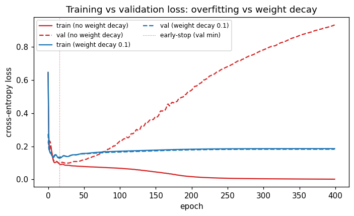
Reading the output. Without regularisation the training loss collapses toward 0 (the 128-128 net memorises the 200 points) while the validation loss bottoms out early and then climbs — textbook overfitting. Weight decay keeps the validation loss lower and flat, trading a little training fit for much better generalisation; early stopping at the validation minimum is a free alternative regulariser.

4. Exercises

1. Replace the cross-entropy with BCEWithLogitsLoss for a single logit output; verify identical AUC.

2. Add a learning-rate scheduler (StepLR).

3. Reproduce on a small image data set (e.g.\ MNIST via torchvision.datasets) — try a CNN.

4. Compare AUC against the LDA / logistic baseline from Chapter 4. Does the MLP win?