
This notebook runs on Colab as-is. The badge link above and the GITHUB_RAW line in the setup cell already point to this repository, so everything installs and loads automatically.
Chapter 7 — Moving Beyond Linearity
Lab: polynomials, splines, LOESS, GAMs
Course: Quantitative Research Methods
Instructor: Prof. Dr. Christoph Weisser, HSBI
Source: James, Witten, Hastie, Tibshirani & Taylor (2023), An Introduction to Statistical Learning, with Applications in Python, Springer. Companion code at statlearning.com.
Goal. Fit increasingly flexible nonlinear regressions on the Wage data; finish with a multivariable GAM.
Setup
Run this cell once. The ISLP package can be installed with pip install ISLP. As an alternative, the same data sets are available as CSVs in the workspace’s ALL CSV FILES - 2nd Edition folder.
Google Colab: this notebook also runs on Colab out of the box — the setup cell below installs any missing packages and downloads the data automatically.
# --- Setup: runs locally AND on Google Colab --------------------------------
# Silence only the spurious 'encountered in matmul' RuntimeWarnings that the macOS
# Accelerate BLAS emits; real warnings (deprecations, model caveats) stay visible.
import warnings
warnings.filterwarnings('ignore', message='.*encountered in matmul', category=RuntimeWarning)
import importlib.util, os, subprocess, sys

IN_COLAB = 'google.colab' in sys.modules

def _ensure(pkg, import_name=None):
    """pip-install pkg (quietly) if its import is missing."""
    if importlib.util.find_spec(import_name or pkg) is None:
        subprocess.run([sys.executable, '-m', 'pip', 'install', '-q', pkg], check=False)

if IN_COLAB:  # Colab ships numpy/pandas/sklearn/statsmodels; add course extras
    for _pkg, _imp in [('ISLP', 'ISLP'), ('pygam', 'pygam')]:
        _ensure(_pkg, _imp)

import numpy as np
import pandas as pd
import matplotlib.pyplot as plt

rng = np.random.default_rng(2024)
plt.rcParams['figure.dpi'] = 110

try:
    from ISLP import load_data
    HAVE_ISLP = True
except ImportError:
    HAVE_ISLP = False
    print('ISLP not installed; using CSV / URL fallbacks.')

# Local CSV location (repo layout first, then legacy paths, then a data/ cache).
_CANDIDATES = ['../ALL CSV FILES - 2nd Edition',
               'ALL CSV FILES - 2nd Edition',
               '../../ALL CSV FILES - 2nd Edition', 'data']
CSV = next((p for p in _CANDIDATES if os.path.isdir(p)), 'data')

# GITHUB_RAW lets a fresh Colab runtime fetch any
# CSV that is neither in ISLP nor already local (spaces in the folder -> %20).
GITHUB_RAW = ('https://raw.githubusercontent.com/ChrisW09/Quantitative-Research-Methods/main/'
              'ALL%20CSV%20FILES%20-%202nd%20Edition')

# The four datasets NOT in the ISLP package -> load from the book's official
# site so the notebook works on a fresh Colab even before the repo is published.
KNOWN_URLS = {
    'Advertising': 'https://www.statlearning.com/s/Advertising.csv',
    'Heart':       'https://www.statlearning.com/s/Heart.csv',
    'Income1':     'https://www.statlearning.com/s/Income1.csv',
    'Income2':     'https://www.statlearning.com/s/Income2.csv',
}

def load(name, **read_csv_kwargs):
    """Load a course dataset. Order: ISLP package -> R datasets -> local CSV
    -> official book URL -> your GitHub repo. Works locally and on Colab."""
    if HAVE_ISLP:
        try:
            return load_data(name)
        except Exception:
            pass
    if name == 'USArrests':                       # classic R dataset, not in ISLP
        try:
            import statsmodels.api as sm
            return sm.datasets.get_rdataset('USArrests', 'datasets').data
        except Exception:
            pass
    path = f'{CSV}/{name}.csv'
    if os.path.exists(path):                      # running from the repo (local)
        return pd.read_csv(path, **read_csv_kwargs)
    remotes = ([KNOWN_URLS[name]] if name in KNOWN_URLS else []) + [f'{GITHUB_RAW}/{name}.csv']
    for url in remotes:                           # fresh Colab: stream over https
        try:
            return pd.read_csv(url, **read_csv_kwargs)
        except Exception:
            continue
    raise FileNotFoundError(
        f"Could not load {name!r}. Put the CSV in '{CSV}/' or check your connection for the GITHUB_RAW fallback.")
1. Polynomial regression
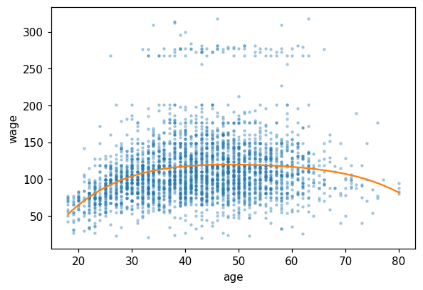
import statsmodels.api as sm
Wage = load('Wage')
from numpy.polynomial import polynomial as P
deg = 4
X = np.column_stack([Wage['age']**d for d in range(deg + 1)])
res = sm.OLS(Wage['wage'], X).fit()
print(res.summary())
                            OLS Regression Results
==============================================================================
Dep. Variable:                   wage   R-squared:                       0.086
Model:                            OLS   Adj. R-squared:                  0.085
Method:                 Least Squares   F-statistic:                     70.69
Date:                Wed, 29 Jul 2026   Prob (F-statistic):           2.77e-57
Time:                        16:51:56   Log-Likelihood:                -15315.
No. Observations:                3000   AIC:                         3.064e+04
Df Residuals:                    2995   BIC:                         3.067e+04
Df Model:                           4
Covariance Type:            nonrobust
==============================================================================
                 coef    std err          t      P>|t|      [0.025      0.975]
------------------------------------------------------------------------------
const       -184.1542     60.040     -3.067      0.002    -301.879     -66.430
x1            21.2455      5.887      3.609      0.000       9.703      32.788
x2            -0.5639      0.206     -2.736      0.006      -0.968      -0.160
x3             0.0068      0.003      2.221      0.026       0.001       0.013
x4         -3.204e-05   1.64e-05     -1.952      0.051   -6.42e-05    1.45e-07
==============================================================================
Omnibus:                     1097.594   Durbin-Watson:                   1.960
Prob(Omnibus):                  0.000   Jarque-Bera (JB):             4965.521
Skew:                           1.722   Prob(JB):                         0.00
Kurtosis:                       8.279   Cond. No.                     5.67e+08
==============================================================================

Notes:
[1] Standard Errors assume that the covariance matrix of the errors is correctly specified.
[2] The condition number is large, 5.67e+08. This might indicate that there are
strong multicollinearity or other numerical problems.
grid = np.linspace(Wage['age'].min(), Wage['age'].max(), 200)
Xg = np.column_stack([grid**d for d in range(deg + 1)])
yhat = res.predict(Xg)
fig, ax = plt.subplots(figsize=(6, 4))
ax.scatter(Wage['age'], Wage['wage'], s=4, alpha=0.3)
ax.plot(grid, yhat, color='C1')
ax.set(xlabel='age', ylabel='wage'); plt.show()
2. Step functions
Wage['age_bin'] = pd.cut(Wage['age'], bins=4)
step = sm.OLS(Wage['wage'], pd.get_dummies(Wage['age_bin']).astype(float)).fit()
print(step.params)
(17.938, 33.5]     94.158392
(33.5, 49.0]      118.211883
(49.0, 64.5]      117.822951
(64.5, 80.0]      101.798984
dtype: float64
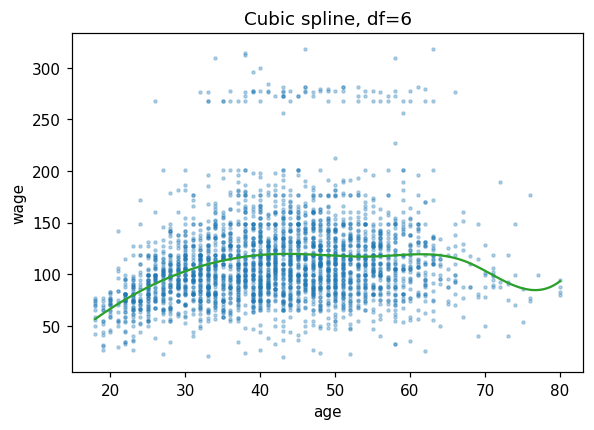
3. Regression splines
from sklearn.preprocessing import SplineTransformer
from sklearn.linear_model import LinearRegression
from sklearn.pipeline import make_pipeline
spl = make_pipeline(SplineTransformer(degree=3, n_knots=6),
                     LinearRegression()).fit(Wage[['age']], Wage['wage'])
# Predict on a DataFrame with the same column name used for the fit; handing
# sklearn a bare array here would drop the feature names and warn.
yhat = spl.predict(pd.DataFrame({'age': grid}))
fig, ax = plt.subplots(figsize=(6, 4))
ax.scatter(Wage['age'], Wage['wage'], s=4, alpha=0.3)
ax.plot(grid, yhat, color='C2')
ax.set(xlabel='age', ylabel='wage', title='Cubic spline, df=6'); plt.show()
4. LOESS
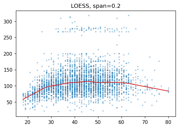
import statsmodels.api as sm
lo = sm.nonparametric.lowess(Wage['wage'], Wage['age'], frac=0.2,
                              return_sorted=True)
fig, ax = plt.subplots(figsize=(6, 4))
ax.scatter(Wage['age'], Wage['wage'], s=4, alpha=0.3)
ax.plot(lo[:, 0], lo[:, 1], color='C3')
ax.set_title('LOESS, span=0.2'); plt.show()
5. GAM
Requires pip install pygam.
try:
    from pygam import LinearGAM, s, f
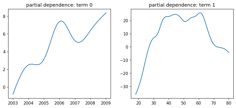
    Xg = Wage[['year', 'age']].values
    yg = Wage['wage'].values
    gam = LinearGAM(s(0) + s(1)).fit(Xg, yg)
    gam.summary()
except ImportError:
    print('pyGAM not installed; pip install pygam')
    gam = None
LinearGAM
=============================================== ==========================================================
Distribution:                        NormalDist Effective DoF:                                     21.1989
Link Function:                     IdentityLink Log Likelihood:                                -24864.6473
Number of Samples:                         3000 AIC:                                            49773.6924
                                                AICc:                                           49774.0384
                                                GCV:                                             1606.4097
                                                Scale:                                           1585.9901
                                                Pseudo R-Squared:                                   0.0953
==========================================================================================================
Feature Function                  Lambda               Rank         EDoF         P > x        Sig. Code
================================= ==================== ============ ============ ============ ============
s(0)                              [0.6]                20           7.1          1.55e-02     *
s(1)                              [0.6]                20           14.1         1.11e-16     ***
intercept                                              1            0.0          1.11e-16     ***
==========================================================================================================
Significance codes:  0 '***' 0.001 '**' 0.01 '*' 0.05 '.' 0.1 ' ' 1

WARNING: Fitting splines and a linear function to a feature introduces a model identifiability problem
         which can cause p-values to appear significant when they are not.

WARNING: p-values calculated in this manner behave correctly for un-penalized models or models with
         known smoothing parameters, but when smoothing parameters have been estimated, the p-values
         are typically lower than they should be, meaning that the tests reject the null too readily.
/var/folders/sz/1k1y5gg975j3mc23vxwrt0v40000gn/T/ipykernel_67560/3808341760.py:6: UserWarning: KNOWN BUG: p-values computed in this summary are likely much smaller than they should be.

Please do not make inferences based on these values!

Collaborate on a solution, and stay up to date at:
github.com/dswah/pyGAM/issues/163

  gam.summary()
if gam is not None:
    fig, axes = plt.subplots(1, 2, figsize=(10, 4))
    for i, ax in enumerate(axes):
        XX = gam.generate_X_grid(term=i)
        ax.plot(XX[:, i], gam.partial_dependence(term=i, X=XX))
        ax.set_title(f'partial dependence: term {i}')
    plt.show()
Lecture exercises — worked Python solutions
These are the [Python] exercises from the lecture slides, solved step by step; run them cell by cell. Data loads through the load() helper defined in the Setup cell, so every cell works locally and on Colab.
Exercise 7.6 — Natural spline / GAM on Wage
Task (from the slides). Using the Wage data:
fit
wageon a natural cubic spline ofagewith 5 df via OLS;fit a GAM
wage ~ s(age) + s(year);describe the estimated effect of
age.
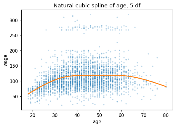
# (a) Natural cubic spline of age with 5 df, fitted by OLS -------------------
# patsy's cr() expands age into 5 natural cubic-spline basis columns
# (natural = linear tails beyond the boundary knots), so this is still
# ordinary least squares -- only the design matrix changes.
import statsmodels.formula.api as smf

Wage = load('Wage')
ns_fit = smf.ols('wage ~ cr(age, df=5)', data=Wage).fit()
print(f'R^2       = {ns_fit.rsquared:.4f}')    # ~0.0871
print(f'F p-value = {ns_fit.f_pvalue:.2e}')    # ~5.9e-58: jointly highly significant

# Plot the fitted spline over the data.
grid_a = pd.DataFrame({'age': np.linspace(Wage['age'].min(), Wage['age'].max(), 200)})
fig, ax = plt.subplots(figsize=(6, 4))
ax.scatter(Wage['age'], Wage['wage'], s=4, alpha=0.2)
ax.plot(grid_a['age'], ns_fit.predict(grid_a), color='C1', lw=2)
ax.set(xlabel='age', ylabel='wage', title='Natural cubic spline of age, 5 df')
plt.show()

# What the output shows: age explains a modest share of wage variance
# (R^2 ~ 0.087), yet the spline terms are jointly overwhelming (p ~ 6e-58).
# Individual cr() basis coefficients are NOT interpretable (the basis columns
# overlap the intercept), so judge the fit by R^2, the F-test and the curve.
R^2       = 0.0872
F p-value = 5.90e-58
# (b) GAM wage ~ s(age) + s(year) with pyGAM ----------------------------------
# Each s() is a penalised smoothing spline; its flexibility is reported as
# effective degrees of freedom (EDF) -- larger EDF = wigglier fitted curve.
from pygam import LinearGAM, s

Xg = Wage[['age', 'year']].values     # column 0 = age, column 1 = year
yg = Wage['wage'].values
gam76 = LinearGAM(s(0) + s(1)).fit(Xg, yg)
gam76.summary()   # with the default penalty: age EDF ~15, year EDF ~6

# Note: pyGAM prints the caveat above. Its summary p-values are a known bug --
# likely much smaller than they should be -- and pyGAM's own advice is not to
# make inferences from them, so ignore the significance stars here.
LinearGAM
=============================================== ==========================================================
Distribution:                        NormalDist Effective DoF:                                     21.1989
Link Function:                     IdentityLink Log Likelihood:                                -24864.6473
Number of Samples:                         3000 AIC:                                            49773.6924
                                                AICc:                                           49774.0384
                                                GCV:                                             1606.4097
                                                Scale:                                           1585.9901
                                                Pseudo R-Squared:                                   0.0953
==========================================================================================================
Feature Function                  Lambda               Rank         EDoF         P > x        Sig. Code
================================= ==================== ============ ============ ============ ============
s(0)                              [0.6]                20           15.2         1.11e-16     ***
s(1)                              [0.6]                20           6.0          1.55e-02     *
intercept                                              1            0.0          1.11e-16     ***
==========================================================================================================
Significance codes:  0 '***' 0.001 '**' 0.01 '*' 0.05 '.' 0.1 ' ' 1

WARNING: Fitting splines and a linear function to a feature introduces a model identifiability problem
         which can cause p-values to appear significant when they are not.

WARNING: p-values calculated in this manner behave correctly for un-penalized models or models with
         known smoothing parameters, but when smoothing parameters have been estimated, the p-values
         are typically lower than they should be, meaning that the tests reject the null too readily.
/var/folders/sz/1k1y5gg975j3mc23vxwrt0v40000gn/T/ipykernel_67560/1112091341.py:9: UserWarning: KNOWN BUG: p-values computed in this summary are likely much smaller than they should be.

Please do not make inferences based on these values!

Collaborate on a solution, and stay up to date at:
github.com/dswah/pyGAM/issues/163

  gam76.summary()   # with the default penalty: age EDF ~15, year EDF ~6
# Partial dependence: the fitted effect of one predictor, the other held fixed.
fig, axes = plt.subplots(1, 2, figsize=(10, 4))
for i, name in enumerate(['age', 'year']):
    XX = gam76.generate_X_grid(term=i)
    axes[i].plot(XX[:, i], gam76.partial_dependence(term=i, X=XX))
    axes[i].set(xlabel=name, ylabel='partial effect on wage')
plt.tight_layout(); plt.show()

# How to read it: the age curve rises steeply to ~40, plateaus between 40 and
# 60, then declines after ~60 -- clearly nonlinear. The year effect is a
# gentle, near-linear upward drift.
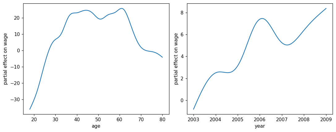
(c) Interpretation. The fitted age effect is clearly nonlinear: wage rises steeply from the late teens to about age 40, is roughly flat between 40 and 60, then declines gently after 60 — a rise–plateau–fall shape that a straight line would miss; this is exactly why a spline/GAM is preferable here. The year effect is a mild, near-linear increase (slow wage growth over the sample window).
Common mistake: interpreting individual spline-basis coefficients (or their t-tests) as “the effect of age” — judge a smooth term by its fitted curve (partial dependence) and by a joint test of all its basis columns.
Extended Exercise 7.3 — Three fits for wage vs. age
Task (from the slides). Model wage as a function of age three ways and compare:
a polynomial, degree chosen by nested ANOVA F-tests (or 5-fold CV);
a step function (bin
ageinto several ranges);a natural cubic spline with about 5 df.
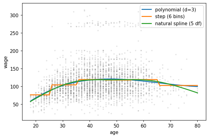
Overlay the three fitted curves on a scatterplot, report the chosen complexity, and interpret where the fits agree and where they differ.
# (1) Choose the polynomial degree by nested ANOVA F-tests -------------------
# Degrees 1..5 give nested models, so each anova_lm row tests d against d+1.
from statsmodels.stats.anova import anova_lm

W = load('Wage')
terms = lambda d: ' + '.join(f'np.power(age, {k})' for k in range(1, d + 1))
models = [smf.ols('wage ~ ' + terms(d), data=W).fit() for d in range(1, 6)]
print(anova_lm(*models)[['df_diff', 'F', 'Pr(>F)']].round(4))

# Reading the table: 2->3 is highly significant (p ~ 0.0017), 3->4 borderline
# (p ~ 0.051), 4->5 clearly insignificant (p ~ 0.37)  =>  choose degree 3.
   df_diff         F  Pr(>F)
0      0.0       NaN     NaN
1      1.0  143.5931  0.0000
2      1.0    9.8888  0.0017
3      1.0    3.8098  0.0510
4      1.0    0.8050  0.3697
# Cross-check with 5-fold CV: test MSE by polynomial degree ------------------
from sklearn.pipeline import make_pipeline
from sklearn.preprocessing import PolynomialFeatures
from sklearn.linear_model import LinearRegression
from sklearn.model_selection import KFold, cross_val_score

for d in range(1, 6):
    pipe = make_pipeline(PolynomialFeatures(d, include_bias=False),
                         LinearRegression())
    cv = -cross_val_score(pipe, W[['age']], W['wage'],
                          cv=KFold(5, shuffle=True, random_state=0),
                          scoring='neg_mean_squared_error')
    print(f'degree {d}: 5-fold CV MSE = {cv.mean():.1f}')

# Expected: ~1676, 1601, 1597, 1596, 1598 -- essentially flat from degree 3 on,
# confirming the ANOVA choice: a cubic is enough.
degree 1: 5-fold CV MSE = 1676.0
degree 2: 5-fold CV MSE = 1600.7
degree 3: 5-fold CV MSE = 1597.0
degree 4: 5-fold CV MSE = 1596.2
degree 5: 5-fold CV MSE = 1598.2
# (2) Step function, (3) natural spline, and the overlay ---------------------
poly = smf.ols('wage ~ ' + terms(3), data=W).fit()           # cubic polynomial
W['bin'] = pd.cut(W['age'], [17, 25, 35, 45, 55, 65, 81])    # six age bins
step = smf.ols('wage ~ C(bin)', data=W).fit()                # step function
ns = smf.ols('wage ~ cr(age, df=5)', data=W).fit()           # natural spline

g = pd.DataFrame({'age': np.arange(18, 81)})                 # prediction grid
g['bin'] = pd.cut(g['age'], [17, 25, 35, 45, 55, 65, 81])    # same cutpoints!

fig, ax = plt.subplots(figsize=(7, 4.5))
ax.scatter(W['age'], W['wage'], s=4, alpha=0.15, color='grey')
for m, lab in [(poly, 'polynomial (d=3)'), (step, 'step (6 bins)'),
               (ns, 'natural spline (5 df)')]:
    ax.plot(g['age'], m.predict(g), lw=2, label=lab)
ax.set(xlabel='age', ylabel='wage'); ax.legend(); plt.show()

print('R^2  poly:', round(poly.rsquared, 4),
      '| step:', round(step.rsquared, 4),
      '| natural spline:', round(ns.rsquared, 4))
# Expected R^2: ~0.0851 | ~0.082 | ~0.0871  (all similar, ~0.08-0.09)
R^2 poly: 0.0851 | step: 0.082 | natural spline: 0.0872
How to read the overlay. In the data-dense interior (ages ≈ 25–70) all three fits trace the same rise–plateau–fall shape. They differ at the sparse boundaries: the polynomial can bend sharply at the extremes, the step function is blocky and discontinuous at its cutpoints, and the natural spline — linear beyond its outer knots — stays smooth and stable at the edges. All three explain a similar share of variance (R² ≈ 0.08–0.09); the natural spline is preferred for its boundary stability.
Common mistake: picking the degree that maximises training R² — it rises mechanically with every added term; only the nested F-tests or CV can tell when the gain is real.
6. Exercises
Fit polynomials of degree 1–5 and use 10-fold CV to pick the best.
Replace the cubic spline with a natural spline (boundary knots = data extrema).
Add
educationas a factor effect in the GAM (LinearGAM(..., f(2))).Reproduce Figure 7.12: per-predictor partial-dependence plots.