This notebook runs on Colab as-is. The badge link above and the GITHUB_RAW line in the setup cell already point to this repository, so everything installs and loads automatically.

Chapter 11 — Survival Analysis

Lab: Kaplan–Meier, log-rank, Cox model with lifelines

Course: Quantitative Research Methods
Instructor: Prof. Dr. Christoph Weisser, HSBI
Source: James, Witten, Hastie, Tibshirani & Taylor (2023), An Introduction to Statistical Learning, with Applications in Python, Springer. Companion code at statlearning.com.

Self-study notebook — a code reference, with no lecture. The lectures cover ISLP chapters 1–8, 10 and 13, so there is no deck for this chapter. Read ISLP Chapter 11 (Survival Analysis) before working through the cells below: this notebook shows how to run the methods in Python, it does not teach the ideas behind them. It also ships without worked solutions — the exercises at the end are left unanswered, for your own practice.

Goal. Plot KM curves, run a log-rank test, and fit a Cox proportional-hazards model on the BrainCancer data. Requires pip install lifelines.

Setup

Run this cell once. The ISLP package can be installed with pip install ISLP. As an alternative, the same data sets are available as CSVs in the workspace’s ALL CSV FILES - 2nd Edition folder.

Google Colab: this notebook also runs on Colab out of the box — the setup cell below installs any missing packages and downloads the data automatically.

# --- Setup: runs locally AND on Google Colab --------------------------------
# Silence only the spurious 'encountered in matmul' RuntimeWarnings that the macOS
# Accelerate BLAS emits; real warnings (deprecations, model caveats) stay visible.
import warnings
warnings.filterwarnings('ignore', message='.*encountered in matmul', category=RuntimeWarning)
import importlib.util, os, subprocess, sys

IN_COLAB = 'google.colab' in sys.modules

def _ensure(pkg, import_name=None):
    """pip-install pkg (quietly) if its import is missing."""
    if importlib.util.find_spec(import_name or pkg) is None:
        subprocess.run([sys.executable, '-m', 'pip', 'install', '-q', pkg], check=False)

if IN_COLAB:  # Colab ships numpy/pandas/sklearn/statsmodels; add course extras
    for _pkg, _imp in [('ISLP', 'ISLP'), ('lifelines', 'lifelines')]:
        _ensure(_pkg, _imp)

import numpy as np
import pandas as pd
import matplotlib.pyplot as plt

rng = np.random.default_rng(2024)
plt.rcParams['figure.dpi'] = 110

try:
    from ISLP import load_data
    HAVE_ISLP = True
except ImportError:
    HAVE_ISLP = False
    print('ISLP not installed; using CSV / URL fallbacks.')

# Local CSV location (repo layout first, then legacy paths, then a data/ cache).
_CANDIDATES = ['../ALL CSV FILES - 2nd Edition',
               'ALL CSV FILES - 2nd Edition',
               '../../ALL CSV FILES - 2nd Edition', 'data']
CSV = next((p for p in _CANDIDATES if os.path.isdir(p)), 'data')

# GITHUB_RAW lets a fresh Colab runtime fetch any
# CSV that is neither in ISLP nor already local (spaces in the folder -> %20).
GITHUB_RAW = ('https://raw.githubusercontent.com/ChrisW09/Quantitative-Research-Methods/main/'
              'ALL%20CSV%20FILES%20-%202nd%20Edition')

# The four datasets NOT in the ISLP package -> load from the book's official
# site so the notebook works on a fresh Colab even before the repo is published.
KNOWN_URLS = {
    'Advertising': 'https://www.statlearning.com/s/Advertising.csv',
    'Heart':       'https://www.statlearning.com/s/Heart.csv',
    'Income1':     'https://www.statlearning.com/s/Income1.csv',
    'Income2':     'https://www.statlearning.com/s/Income2.csv',
}

def load(name, **read_csv_kwargs):
    """Load a course dataset. Order: ISLP package -> R datasets -> local CSV
    -> official book URL -> your GitHub repo. Works locally and on Colab."""
    if HAVE_ISLP:
        try:
            return load_data(name)
        except Exception:
            pass
    if name == 'USArrests':                       # classic R dataset, not in ISLP
        try:
            import statsmodels.api as sm
            return sm.datasets.get_rdataset('USArrests', 'datasets').data
        except Exception:
            pass
    path = f'{CSV}/{name}.csv'
    if os.path.exists(path):                      # running from the repo (local)
        return pd.read_csv(path, **read_csv_kwargs)
    remotes = ([KNOWN_URLS[name]] if name in KNOWN_URLS else []) + [f'{GITHUB_RAW}/{name}.csv']
    for url in remotes:                           # fresh Colab: stream over https
        try:
            return pd.read_csv(url, **read_csv_kwargs)
        except Exception:
            continue
    raise FileNotFoundError(
        f"Could not load {name!r}. Put the CSV in '{CSV}/' or check your connection for the GITHUB_RAW fallback.")

1. Data

BC = load('BrainCancer', index_col=0)   # CSV carries a row-number column
BC = BC.dropna().reset_index(drop=True)
BC.head()

	sex	diagnosis	loc	ki	gtv	stereo	status	time
0	Female	Meningioma	Infratentorial	90	6.11	SRS	0	57.64
1	Male	HG glioma	Supratentorial	90	19.35	SRT	1	8.98
2	Female	Meningioma	Infratentorial	70	7.95	SRS	0	26.46
3	Female	LG glioma	Supratentorial	80	7.61	SRT	1	47.80
4	Male	HG glioma	Supratentorial	90	5.06	SRT	1	6.30

2. Kaplan-Meier

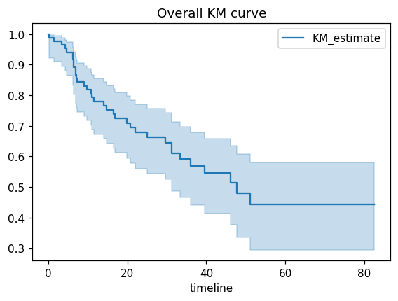
from lifelines import KaplanMeierFitter, CoxPHFitter
from lifelines.statistics import logrank_test
km = KaplanMeierFitter().fit(BC['time'], BC['status'])
fig, ax = plt.subplots(figsize=(6, 4))
km.plot_survival_function(ax=ax); ax.set_title('Overall KM curve')
plt.show()

Stratified by sex

fig, ax = plt.subplots(figsize=(6, 4))
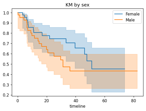
for sex in BC['sex'].unique():
    mask = BC['sex'] == sex
    KaplanMeierFitter().fit(BC.loc[mask, 'time'],
                              BC.loc[mask, 'status'], label=sex)\
        .plot_survival_function(ax=ax)
ax.set_title('KM by sex'); plt.show()

3. Log-rank test

m = BC['sex'] == 'Male'
res = logrank_test(BC.loc[m, 'time'],  BC.loc[~m, 'time'],
                    BC.loc[m, 'status'], BC.loc[~m, 'status'])
print('log-rank statistic :', round(res.test_statistic, 2))
print('p-value           :', round(res.p_value, 4))

log-rank statistic : 1.79
p-value           : 0.1814

4. Cox proportional-hazards model

df = pd.get_dummies(BC, drop_first=True).astype(float)
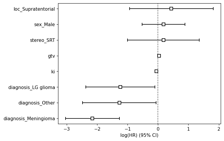
cph = CoxPHFitter().fit(df, duration_col='time', event_col='status')
cph.print_summary()

model	lifelines.CoxPHFitter
duration col	'time'
event col	'status'
baseline estimation	breslow
number of observations	87
number of events observed	35
partial log-likelihood	-116.75
time fit was run	2026-07-19 12:32:30 UTC

	coef	exp(coef)	se(coef)	coef lower 95%	coef upper 95%	exp(coef) lower 95%	exp(coef) upper 95%	cmp to	z	p	-log2(p)
ki	-0.05	0.95	0.02	-0.09	-0.02	0.91	0.98	0.00	-3.00	<0.005	8.54
gtv	0.03	1.03	0.02	-0.01	0.08	0.99	1.08	0.00	1.54	0.12	3.00
sex_Male	0.18	1.20	0.36	-0.52	0.89	0.59	2.44	0.00	0.51	0.61	0.71
diagnosis_LG glioma	-1.24	0.29	0.58	-2.38	-0.10	0.09	0.90	0.00	-2.14	0.03	4.95
diagnosis_Meningioma	-2.15	0.12	0.45	-3.04	-1.27	0.05	0.28	0.00	-4.78	<0.005	19.14
diagnosis_Other	-1.27	0.28	0.62	-2.48	-0.06	0.08	0.94	0.00	-2.05	0.04	4.65
loc_Supratentorial	0.44	1.55	0.70	-0.94	1.82	0.39	6.17	0.00	0.63	0.53	0.91
stereo_SRT	0.18	1.19	0.60	-1.00	1.36	0.37	3.88	0.00	0.30	0.77	0.38

Concordance	0.79
Partial AIC	249.50
log-likelihood ratio test	41.37 on 8 df
-log2(p) of ll-ratio test	19.10

cph.plot()
plt.show()

5. Exercises

1. Compute the C-index of the Cox model.

2. Add an interaction term in the Cox fit and test its significance.

3. Use lifelines.WeibullAFTFitter for a parametric alternative.

4. Repeat on the Publication data set and discuss differences.