This notebook runs on Colab as-is. The badge link above and the GITHUB_RAW line in the setup cell already point to this repository, so everything installs and loads automatically.

Chapter 9 — Support Vector Machines

Lab: linear, polynomial, and radial-kernel SVMs

Course: Quantitative Research Methods
Instructor: Prof. Dr. Christoph Weisser, HSBI
Source: James, Witten, Hastie, Tibshirani & Taylor (2023), An Introduction to Statistical Learning, with Applications in Python, Springer. Companion code at statlearning.com.

Self-study notebook — a code reference, with no lecture. The lectures cover ISLP chapters 1–8, 10 and 13, so there is no deck for this chapter. Read ISLP Chapter 9 (Support Vector Machines) before working through the cells below: this notebook shows how to run the methods in Python, it does not teach the ideas behind them. It also ships without worked solutions — the exercises at the end are left unanswered, for your own practice.

Goal. Fit linear and kernel SVMs on a 2-D toy data set, visualise the decision boundary, and tune \(C\) and \(\gamma\).

Setup

Run this cell once. The ISLP package can be installed with pip install ISLP. As an alternative, the same data sets are available as CSVs in the workspace’s ALL CSV FILES - 2nd Edition folder.

Google Colab: this notebook also runs on Colab out of the box — the setup cell below installs any missing packages and downloads the data automatically.

# --- Setup: runs locally AND on Google Colab --------------------------------
# Silence only the spurious 'encountered in matmul' RuntimeWarnings that the macOS
# Accelerate BLAS emits; real warnings (deprecations, model caveats) stay visible.
import warnings
warnings.filterwarnings('ignore', message='.*encountered in matmul', category=RuntimeWarning)
import importlib.util, os, subprocess, sys

IN_COLAB = 'google.colab' in sys.modules

def _ensure(pkg, import_name=None):
    """pip-install pkg (quietly) if its import is missing."""
    if importlib.util.find_spec(import_name or pkg) is None:
        subprocess.run([sys.executable, '-m', 'pip', 'install', '-q', pkg], check=False)

if IN_COLAB:  # Colab ships numpy/pandas/sklearn/statsmodels; add course extras
    for _pkg, _imp in [('ISLP', 'ISLP')]:
        _ensure(_pkg, _imp)

import numpy as np
import pandas as pd
import matplotlib.pyplot as plt

rng = np.random.default_rng(2024)
plt.rcParams['figure.dpi'] = 110

try:
    from ISLP import load_data
    HAVE_ISLP = True
except ImportError:
    HAVE_ISLP = False
    print('ISLP not installed; using CSV / URL fallbacks.')

# Local CSV location (repo layout first, then legacy paths, then a data/ cache).
_CANDIDATES = ['../ALL CSV FILES - 2nd Edition',
               'ALL CSV FILES - 2nd Edition',
               '../../ALL CSV FILES - 2nd Edition', 'data']
CSV = next((p for p in _CANDIDATES if os.path.isdir(p)), 'data')

# GITHUB_RAW lets a fresh Colab runtime fetch any
# CSV that is neither in ISLP nor already local (spaces in the folder -> %20).
GITHUB_RAW = ('https://raw.githubusercontent.com/ChrisW09/Quantitative-Research-Methods/main/'
              'ALL%20CSV%20FILES%20-%202nd%20Edition')

# The four datasets NOT in the ISLP package -> load from the book's official
# site so the notebook works on a fresh Colab even before the repo is published.
KNOWN_URLS = {
    'Advertising': 'https://www.statlearning.com/s/Advertising.csv',
    'Heart':       'https://www.statlearning.com/s/Heart.csv',
    'Income1':     'https://www.statlearning.com/s/Income1.csv',
    'Income2':     'https://www.statlearning.com/s/Income2.csv',
}

def load(name, **read_csv_kwargs):
    """Load a course dataset. Order: ISLP package -> R datasets -> local CSV
    -> official book URL -> your GitHub repo. Works locally and on Colab."""
    if HAVE_ISLP:
        try:
            return load_data(name)
        except Exception:
            pass
    if name == 'USArrests':                       # classic R dataset, not in ISLP
        try:
            import statsmodels.api as sm
            return sm.datasets.get_rdataset('USArrests', 'datasets').data
        except Exception:
            pass
    path = f'{CSV}/{name}.csv'
    if os.path.exists(path):                      # running from the repo (local)
        return pd.read_csv(path, **read_csv_kwargs)
    remotes = ([KNOWN_URLS[name]] if name in KNOWN_URLS else []) + [f'{GITHUB_RAW}/{name}.csv']
    for url in remotes:                           # fresh Colab: stream over https
        try:
            return pd.read_csv(url, **read_csv_kwargs)
        except Exception:
            continue
    raise FileNotFoundError(
        f"Could not load {name!r}. Put the CSV in '{CSV}/' or check your connection for the GITHUB_RAW fallback.")

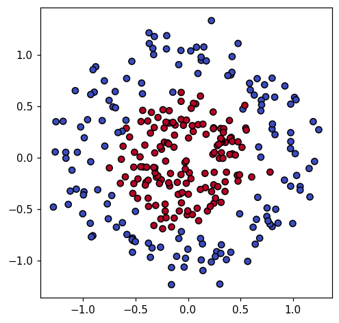
1. Synthetic two-class data

from sklearn.datasets import make_circles
X, y = make_circles(n_samples=300, factor=0.4, noise=0.15, random_state=0)
fig, ax = plt.subplots(figsize=(5, 5))
ax.scatter(X[:, 0], X[:, 1], c=y, cmap='coolwarm', edgecolor='k')
plt.show()

2. Linear SVM

from sklearn.svm import SVC
from sklearn.preprocessing import StandardScaler
from sklearn.pipeline import make_pipeline
from sklearn.model_selection import GridSearchCV
lin = make_pipeline(StandardScaler(), SVC(kernel='linear'))
lin_g = GridSearchCV(lin, {'svc__C': np.logspace(-2, 2, 9)}, cv=5).fit(X, y)
print('best C:', lin_g.best_params_, '  CV acc:', round(lin_g.best_score_, 3))

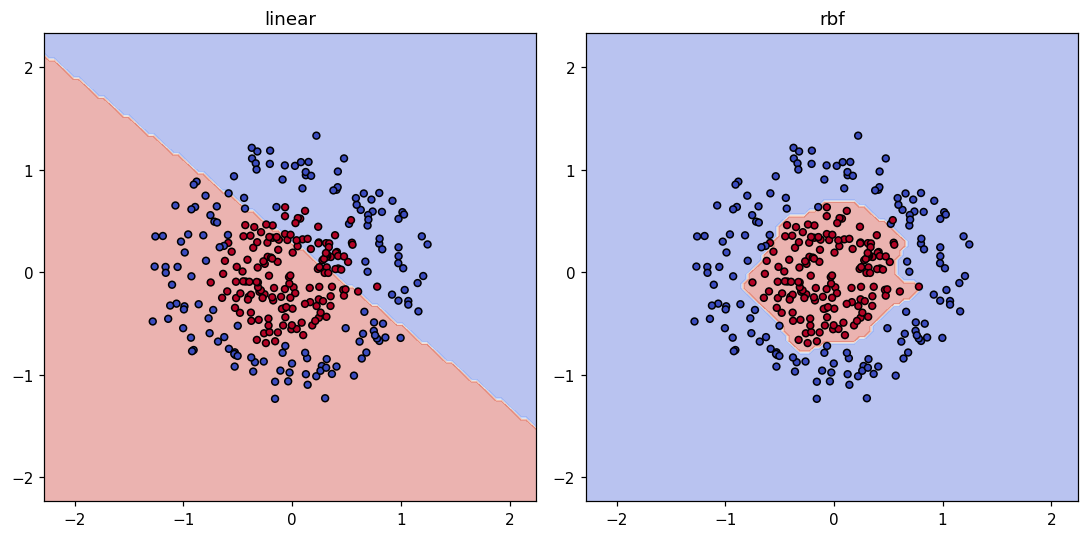
best C: {'svc__C': np.float64(0.01)}   CV acc: 0.583

3. Radial-kernel SVM

rbf = make_pipeline(StandardScaler(), SVC(kernel='rbf'))
rbf_g = GridSearchCV(rbf,
        {'svc__C': np.logspace(-2, 2, 5),
         'svc__gamma': np.logspace(-3, 1, 5)}, cv=5).fit(X, y)
print('best params:', rbf_g.best_params_,
      '  CV acc:', round(rbf_g.best_score_, 3))

best params: {'svc__C': np.float64(1.0), 'svc__gamma': np.float64(10.0)}   CV acc: 0.98

Decision boundary

from sklearn.inspection import DecisionBoundaryDisplay
fig, axes = plt.subplots(1, 2, figsize=(10, 5))
for ax, name, mdl in [(axes[0], 'linear', lin_g.best_estimator_),
                       (axes[1], 'rbf',   rbf_g.best_estimator_)]:
    DecisionBoundaryDisplay.from_estimator(mdl, X, ax=ax,
        response_method='predict', alpha=0.4, cmap='coolwarm')
    ax.scatter(X[:, 0], X[:, 1], c=y, cmap='coolwarm', edgecolor='k', s=20)
    ax.set_title(name)
plt.tight_layout(); plt.show()

4. Real data: Heart

# Heart is not in the ISLP package, so load() falls back to the CSV, whose
# first (unnamed) column is just the row number -> index_col=0 keeps it out
# of the design matrix.
Heart = load('Heart', index_col=0).dropna().reset_index(drop=True)
y = (Heart['AHD'] == 'Yes').astype(int).values
X = pd.get_dummies(Heart.drop(columns='AHD'), drop_first=True).astype(float).values
from sklearn.model_selection import train_test_split
Xtr, Xte, ytr, yte = train_test_split(X, y, test_size=0.3, random_state=0)
rbf = make_pipeline(StandardScaler(), SVC(kernel='rbf', C=1, gamma=0.05)).fit(Xtr, ytr)
print('test acc:', rbf.score(Xte, yte))

test acc: 0.8222222222222222

5. Exercises

1. Compare radial SVM with logistic regression on the Heart data.

2. Plot ROC curves for SVM and logistic regression.

3. Try a polynomial kernel of degree 2 on make_circles. Does it match the radial kernel?

4. Use Platt scaling (SVC(probability=True)) to obtain calibrated probabilities; check the calibration curve.