
This notebook runs on Colab as-is. The badge link above and the GITHUB_RAW line in the setup cell already point to this repository, so everything installs and loads automatically.
Chapter 8 — Tree-Based Methods
Lab: trees, random forests, gradient boosting, XGBoost
Course: Quantitative Research Methods
Instructor: Prof. Dr. Christoph Weisser, HSBI
Source: James, Witten, Hastie, Tibshirani & Taylor (2023), An Introduction to Statistical Learning, with Applications in Python, Springer. Companion code at statlearning.com.
Goal. Fit a single regression tree on Carseats, then bagging, random forests, and gradient boosting; compare test errors.
Setup
Run this cell once. The ISLP package can be installed with pip install ISLP. As an alternative, the same data sets are available as CSVs in the workspace’s ALL CSV FILES - 2nd Edition folder.
Google Colab: this notebook also runs on Colab out of the box — the setup cell below installs any missing packages and downloads the data automatically.
# --- Setup: runs locally AND on Google Colab --------------------------------
# Silence only the spurious 'encountered in matmul' RuntimeWarnings that the macOS
# Accelerate BLAS emits; real warnings (deprecations, model caveats) stay visible.
import warnings
warnings.filterwarnings('ignore', message='.*encountered in matmul', category=RuntimeWarning)
import importlib.util, os, subprocess, sys

IN_COLAB = 'google.colab' in sys.modules

def _ensure(pkg, import_name=None):
    """pip-install pkg (quietly) if its import is missing."""
    if importlib.util.find_spec(import_name or pkg) is None:
        subprocess.run([sys.executable, '-m', 'pip', 'install', '-q', pkg], check=False)

if IN_COLAB:  # Colab ships numpy/pandas/sklearn/statsmodels; add course extras
    for _pkg, _imp in [('ISLP', 'ISLP'), ('xgboost', 'xgboost')]:
        _ensure(_pkg, _imp)

import numpy as np
import pandas as pd
import matplotlib.pyplot as plt

rng = np.random.default_rng(2024)
plt.rcParams['figure.dpi'] = 110

try:
    from ISLP import load_data
    HAVE_ISLP = True
except ImportError:
    HAVE_ISLP = False
    print('ISLP not installed; using CSV / URL fallbacks.')

# Local CSV location (repo layout first, then legacy paths, then a data/ cache).
_CANDIDATES = ['../ALL CSV FILES - 2nd Edition',
               'ALL CSV FILES - 2nd Edition',
               '../../ALL CSV FILES - 2nd Edition', 'data']
CSV = next((p for p in _CANDIDATES if os.path.isdir(p)), 'data')

# GITHUB_RAW lets a fresh Colab runtime fetch any
# CSV that is neither in ISLP nor already local (spaces in the folder -> %20).
GITHUB_RAW = ('https://raw.githubusercontent.com/ChrisW09/Quantitative-Research-Methods/main/'
              'ALL%20CSV%20FILES%20-%202nd%20Edition')

# The four datasets NOT in the ISLP package -> load from the book's official
# site so the notebook works on a fresh Colab even before the repo is published.
KNOWN_URLS = {
    'Advertising': 'https://www.statlearning.com/s/Advertising.csv',
    'Heart':       'https://www.statlearning.com/s/Heart.csv',
    'Income1':     'https://www.statlearning.com/s/Income1.csv',
    'Income2':     'https://www.statlearning.com/s/Income2.csv',
}

def load(name, **read_csv_kwargs):
    """Load a course dataset. Order: ISLP package -> R datasets -> local CSV
    -> official book URL -> your GitHub repo. Works locally and on Colab."""
    if HAVE_ISLP:
        try:
            return load_data(name)
        except Exception:
            pass
    if name == 'USArrests':                       # classic R dataset, not in ISLP
        try:
            import statsmodels.api as sm
            return sm.datasets.get_rdataset('USArrests', 'datasets').data
        except Exception:
            pass
    path = f'{CSV}/{name}.csv'
    if os.path.exists(path):                      # running from the repo (local)
        return pd.read_csv(path, **read_csv_kwargs)
    remotes = ([KNOWN_URLS[name]] if name in KNOWN_URLS else []) + [f'{GITHUB_RAW}/{name}.csv']
    for url in remotes:                           # fresh Colab: stream over https
        try:
            return pd.read_csv(url, **read_csv_kwargs)
        except Exception:
            continue
    raise FileNotFoundError(
        f"Could not load {name!r}. Put the CSV in '{CSV}/' or check your connection for the GITHUB_RAW fallback.")
1. The Carseats data
Carseats = load('Carseats')
X = pd.get_dummies(Carseats.drop(columns='Sales'), drop_first=True).astype(float)
y = Carseats['Sales']
from sklearn.model_selection import train_test_split
Xtr, Xte, ytr, yte = train_test_split(X, y, test_size=0.3, random_state=0)
print(X.shape)
(400, 11)
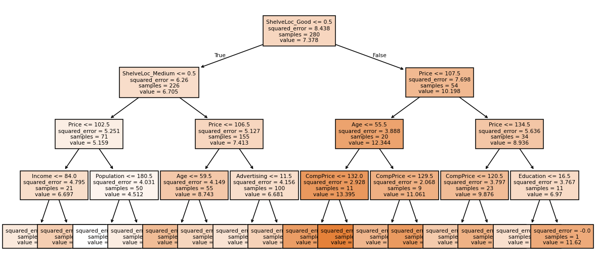
2. Single regression tree
from sklearn.tree import DecisionTreeRegressor, plot_tree
tree = DecisionTreeRegressor(max_depth=4, random_state=0).fit(Xtr, ytr)
fig, ax = plt.subplots(figsize=(13, 6))
plot_tree(tree, feature_names=X.columns, filled=True, fontsize=7, ax=ax)
plt.show()
print('test MSE single tree:', ((yte - tree.predict(Xte))**2).mean().round(3))
test MSE single tree: 3.612
3. Pruning via cost-complexity
from sklearn.model_selection import GridSearchCV
grid = GridSearchCV(DecisionTreeRegressor(random_state=0),
                     {'ccp_alpha': np.linspace(0, 0.05, 20)},
                     cv=10, scoring='neg_mean_squared_error').fit(Xtr, ytr)
print('best alpha :', round(grid.best_params_['ccp_alpha'], 4))
print('test MSE   :', ((yte - grid.best_estimator_.predict(Xte))**2).mean().round(3))
best alpha : 0.0132
test MSE   : 4.62
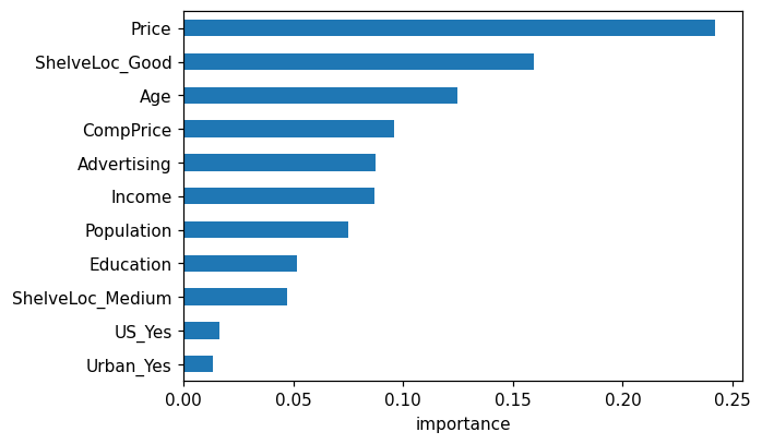
4. Random forest
from sklearn.ensemble import RandomForestRegressor
rf = RandomForestRegressor(n_estimators=500, max_features='sqrt',
                            random_state=0, oob_score=True).fit(Xtr, ytr)
print('OOB R^2 :', round(rf.oob_score_, 3))
print('test MSE :', ((yte - rf.predict(Xte))**2).mean().round(3))
OOB R^2 : 0.629
test MSE : 2.312
imp = pd.Series(rf.feature_importances_, index=X.columns).sort_values()
fig, ax = plt.subplots(figsize=(6, 4))
imp.plot.barh(ax=ax); ax.set_xlabel('importance'); plt.show()
5. Gradient boosting
from sklearn.ensemble import GradientBoostingRegressor
gb = GradientBoostingRegressor(n_estimators=2000, learning_rate=0.01,
                                max_depth=3, random_state=0).fit(Xtr, ytr)
print('test MSE :', ((yte - gb.predict(Xte))**2).mean().round(3))
test MSE : 2.195
Optional: XGBoost
try:
    import xgboost as xgb
    bst = xgb.XGBRegressor(n_estimators=2000, learning_rate=0.05,
                            max_depth=4, subsample=0.8, random_state=0).fit(Xtr, ytr)
    print('XGBoost test MSE :', ((yte - bst.predict(Xte))**2).mean().round(3))
except ImportError:
    print('xgboost not installed; pip install xgboost')
XGBoost test MSE : 2.249
Lecture exercises — worked Python solutions
These are the [Python] exercises from the lecture slides, solved step by step; run them cell by cell. Data loads through the load() helper defined in the Setup cell, so every cell works locally and on Colab.
Exercise 8.7 — Random forest & boosting on Boston
Task (from the slides). Using the Boston data (target medv):
fit a random forest and a gradient-boosting regressor; report test MSE;
read off the most important features from the random forest;
interpret the result.
# (a) Load Boston and make a reproducible 70/30 train/test split -------------
from sklearn.ensemble import RandomForestRegressor, GradientBoostingRegressor
from sklearn.model_selection import train_test_split
from sklearn.metrics import mean_squared_error

Boston = load('Boston')
Boston = Boston.drop(columns=[c for c in ['Unnamed: 0'] if c in Boston.columns])
Xb = Boston.drop(columns='medv')      # 12 predictors
yb = Boston['medv']                   # median home value (in $1000s)
Xtr_b, Xte_b, ytr_b, yte_b = train_test_split(Xb, yb, test_size=0.3,
                                              random_state=0)
print('train:', Xtr_b.shape, ' test:', Xte_b.shape)   # (354, 12) / (152, 12)
train: (354, 12) test: (152, 12)
# Fit both ensembles and compare held-out test MSE ----------------------------
rf = RandomForestRegressor(n_estimators=500, max_features='sqrt',  # B=500, m=sqrt(p)
                           random_state=0).fit(Xtr_b, ytr_b)
print('RF  test MSE:',
      round(mean_squared_error(yte_b, rf.predict(Xte_b)), 2))   # ~19.6

gb = GradientBoostingRegressor(n_estimators=1000, learning_rate=0.01,  # slow learning
                               max_depth=3, random_state=0).fit(Xtr_b, ytr_b)
print('GBM test MSE:',
      round(mean_squared_error(yte_b, gb.predict(Xte_b)), 2))   # ~13.5
RF  test MSE: 19.65
GBM test MSE: 13.46
# (b) Random-forest variable importance ---------------------------------------
# feature_importances_ = total impurity (RSS) reduction per variable, summed
# over all splits of all 500 trees and normalised to sum to 1.
imp_b = pd.Series(rf.feature_importances_,
                  index=Xb.columns).sort_values(ascending=False)
print(imp_b.round(3).head())          # lstat ~0.28 and rm ~0.27 dominate

imp_b.sort_values().plot.barh(figsize=(6, 4))
plt.xlabel('importance'); plt.tight_layout(); plt.show()
lstat      0.279
rm         0.267
indus      0.079
ptratio    0.077
crim       0.066
dtype: float64
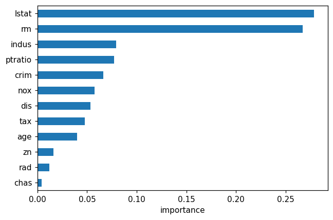
(c) What the output shows. Both ensembles land far below a single unpruned tree (test MSE ≈ 27 on this split): boosting reaches ≈ 13.5 and the m=√p forest ≈ 19.6. Boston has a few dominant predictors, so restricting each split to √12 ≈ 3 candidate features hurts the forest on this particular split — Extended Exercise 8.3 below shows that a larger max_features closes the gap. The importance ranking is headed by lstat (% lower-status population, ≈ 0.28) and rm (average rooms per dwelling, ≈ 0.27): housing value is driven mostly by neighbourhood socio-economic status and dwelling size.
Extended Exercise 8.3 — Bagging vs. random forest vs. boosting
Task (from the slides). Using Boston (target medv), fit and compare three ensembles against a single tree:
bagging (a forest that considers all p predictors at each split);
a random forest, tuning m = features tried per split;
gradient boosting, tuning (B, λ, d) = (trees, learning rate, depth).
Report the test MSE of each, and read off the random-forest variable-importance ranking. Which method wins, and which predictors matter?
# (1) Single deep tree vs. bagging (fresh split, seed 1 as in the lecture) ---
from sklearn.tree import DecisionTreeRegressor

p = Xb.shape[1]                                                # p = 12
Xtr8, Xte8, ytr8, yte8 = train_test_split(Xb, yb, test_size=0.3,
                                          random_state=1)

tree8 = DecisionTreeRegressor(random_state=1).fit(Xtr8, ytr8)  # unpruned tree
bag8 = RandomForestRegressor(n_estimators=500, max_features=p, # m = p -> bagging
                             random_state=1).fit(Xtr8, ytr8)
print('single tree test MSE:',
      round(mean_squared_error(yte8, tree8.predict(Xte8)), 2))   # ~26.7
print('bagging     test MSE:',
      round(mean_squared_error(yte8, bag8.predict(Xte8)), 2))    # ~8.5
# Averaging 500 bootstrap trees removes most of the single tree's error -- though
# this tree seed flatters the ensemble; see the discussion at the end.
single tree test MSE: 26.67
bagging     test MSE: 8.56
# (2) Random forest: tune m = max_features (candidates per split) -------------
# Choose m by 5-fold CV *inside the training set*; picking the m with the
# smallest TEST MSE would make the test set part of the fitting process and the
# reported error optimistic.  The test set is scored once, for the winner only.
from sklearn.model_selection import GridSearchCV

rf_cv = GridSearchCV(RandomForestRegressor(n_estimators=500, random_state=1),
                     {'max_features': ['sqrt', 4, 6]},
                     cv=5, scoring='neg_mean_squared_error').fit(Xtr8, ytr8)
for m, s in zip(rf_cv.cv_results_['param_max_features'],
                -rf_cv.cv_results_['mean_test_score']):
    print(f'RF max_features={str(m):>4}: CV MSE = {s:.2f}')
# Expected: sqrt ~13.2, 4 ~12.5, 6 ~11.9  ->  a larger m helps on Boston because
# its few strong predictors (lstat, rm) should be available at most splits.

rf8 = rf_cv.best_estimator_                      # already re-fit on all of Xtr8
print('chosen m :', rf_cv.best_params_['max_features'],
      '-> test MSE =', round(mean_squared_error(yte8, rf8.predict(Xte8)), 2))  # 6 -> ~8.7
RF max_features=sqrt: CV MSE = 13.24
RF max_features=   4: CV MSE = 12.52
RF max_features=   6: CV MSE = 11.91
chosen m : 6 -> test MSE = 8.73
# (3) Gradient boosting: tune (learning rate, number of trees, depth) ---------
# Same rule as above: the winning setting is chosen on training-set CV, and only
# that one model is then scored on the test set.
gbm_grid = [{'learning_rate': [0.1],  'n_estimators': [1000], 'max_depth': [2]},
            {'learning_rate': [0.01], 'n_estimators': [2000], 'max_depth': [3]}]
gbm_cv = GridSearchCV(GradientBoostingRegressor(random_state=1), gbm_grid,
                      cv=5, scoring='neg_mean_squared_error').fit(Xtr8, ytr8)
for prm, s in zip(gbm_cv.cv_results_['params'],
                  -gbm_cv.cv_results_['mean_test_score']):
    print(f"GBM lr={prm['learning_rate']}, B={prm['n_estimators']}, "
          f"depth={prm['max_depth']}: CV MSE = {s:.2f}")
# Expected: (0.1, 1000, 2) ~15.8 and (0.01, 2000, 3) ~10.9
#           ->  slow learning with many trees wins.

gbm8 = gbm_cv.best_estimator_
print('chosen   :', gbm_cv.best_params_)
print('test MSE :', round(mean_squared_error(yte8, gbm8.predict(Xte8)), 2))   # ~7.3
GBM lr=0.1, B=1000, depth=2: CV MSE = 15.78
GBM lr=0.01, B=2000, depth=3: CV MSE = 10.92
chosen   : {'learning_rate': 0.01, 'max_depth': 3, 'n_estimators': 2000}
test MSE : 7.34
# Variable importance of the tuned (max_features=6) forest --------------------
imp8 = pd.Series(rf8.feature_importances_,
                 index=Xb.columns).sort_values(ascending=False)
print(imp8.round(3).head())
# lstat (~0.40) and rm (~0.27) dominate, then dis and nox.
# (Magnitudes shift slightly across sklearn versions; the ranking is stable.)
lstat    0.400
rm       0.270
dis      0.069
nox      0.054
crim     0.052
dtype: float64
What the numbers say. On this split (seed 1): single tree ≈ 26.7 → bagging ≈ 8.6. For the forest, 5-fold CV inside the training set prefers m = 6 (CV MSE ≈ 11.9, against ≈ 13.2 at m=√p), and that chosen model then scores ≈ 8.7 on the test set; boosting’s CV likewise prefers slow learning (λ=0.01, B=2000, d=3: CV MSE ≈ 10.9 against ≈ 15.8), reaching ≈ 7.3 on test — so well-tuned boosting wins. Note where the hyperparameters were chosen: comparing test MSEs to pick m or (λ, B, d) would make the test set part of the fitting process, so selection runs on training-set CV and the test set is scored once per method. The realistic gain from ensembling here is about two-fold, not the three-fold ratio the printed numbers suggest — a fully grown single tree is by far the noisiest model in the comparison, and random_state=1 happens to grow one of its worse trees on this split, so other tree seeds and newer scikit-learn versions put the single tree well below 26.7 while every ensemble number barely budges. Because Boston has few, strong predictors, a larger m helps the forest — which is why plain bagging (m=p) is competitive here. The importance ranking (lstat, rm, then dis, nox) says housing value is driven mostly by neighbourhood socio-economic status and dwelling size. Boosting needs tuning; the random forest remains the strong low-effort default.
6. Exercises
Tune the random forest’s
max_features. What value wins on CV?Tune the gradient booster’s learning rate, depth, and
n_estimatorsjointly.Use permutation importance instead of impurity importance.
Replace Carseats with the OJ data and predict
Purchase. Report test accuracy.